This activity walks you through the use of very simple machine learning (K-Nearest Neighbor) for a computer vision task, and then teaches you how to use the Tensorflow library to train an image classifier, and the YOLO library to finetune an object detection network. We will use Google Colab to train the deep learning models.
The Github repository for this assignment will contain starter code for the simple machine learning examples
The first two tasks are examples of image classification. Image classification is a straightforward task, where we input an image, and the network assigns a category to it. For example, we might want to classify images according to what kind of vehicle is in them: car, truck, bicycle, train, etc. Or we might want to classify images of handwritten letters or digits by what letter or digit they contain.
The third task looks at a more complex problem: object detection. Here, we go beyond a category for the entire image. Instead, we locate objects within the image and mark them with a rectangular bounding box, and categorize each object found.
You can install Tensorflow and YOLO on your own computer. However, the training time with CPU only will be ridiculously long, and it often takes days to correctly set up your computer so that these libraries can use your GPU, if it is possible at all.
K-Nearest Neighbor
Creating artificial data
The code below, adapted from the OpenCV Machine Learning tutorial, generates random data, and assigns half of them to one category and the other half to a second category. It then generates a new random value. It plots this data as a scatterplot (note: you must close the plot window for the program to go on).
import osimport randomimport timeimport cv2import numpy as npfrom sklearn.model_selection import train_test_splitimport matplotlib.pyplot as plt # Used to display plots and chart of data (and sometimes images)def plotDataAndPoint(data, categ, newPoints):"""Takes in data and a list of responses, as well as a list of new points, and it creates a scatter plot red triangles: data with categ = 0 blue squares: data with categ = 1 green circles: unknown data""" red = data[categ==0] # this selects just data where bool is true plt.scatter(red[:, 0], red[:, 1], 80, 'r', '^') blue = data[categ==1] plt.scatter(blue[:, 0], blue[:, 1], 80, 'b', 's')# Plot a new point in green plt.scatter(newPoints[:, 0], newPoint[:, 1], 80, 'g', 'o') plt.show()trainData = np.random.randint(0, 100, (40, 2)).astype(np.float32)trainLabels = np.random.randint(0, 2, 40).astype(np.float32)# Generate a new pointnewPoint = np.random.randint(0, 100, (1, 2)).astype(np.float32)# Plot random data, and new (random) pointplotDataAndPoint(trainData, trainLabels, newPoint)
1
Create a float matrix with 40 rows and 2 columns, filled with random values between 0 and 100: (x, y) coordinates
2
Create a float array with 40 rows, filled with random 0’s and 1s: the two categories we want it to learn
3
Generate a new float matrix that has 1 row and 2 columns, with random values between 0 and 100: this is our unknown point. Note that we can also generate multiple unknown points to test by increasing the number of rows
4
Plot the data
5
Select the rows from the data where the corresponding category value is 0, and plot them with red triangles
6
Select the rows from the data where the corresponding category value is 1, and plot them with blue squares
7
Plot the unknown point(s) as green circles
8
To see the window, you must call plt.show
/Library/Frameworks/Python.framework/Versions/3.12/lib/python3.12/site-packages/sklearn/utils/_param_validation.py:11: UserWarning:

A NumPy version >=1.23.5 and <2.3.0 is required for this version of SciPy (detected version 2.3.1)
Building and training a KNN model
OpenCV implements several simple ML models, including KNN.
Here we set up the KNN model as a n object, and train it on the data from the previous section:
# Create KNN object and train on dataknn = cv2.ml.KNearest_create()knn.train(trainData, cv2.ml.ROW_SAMPLE, trainLabels)
1
We pass in the training data, a constant that indicates where the instances are organized in rows or columns, and then the labels, or categories, for the data
True
Classifying the unknown point
Next we run the trained model on our new point, and see the results.
# Report category of new point (based on k=3)ret, result, neighbors, dist = knn.findNearest(newPoint, 3)print("ret:", ret)print("result:", result)print("neighbors:", neighbors)print("distances:", dist)
1
Calls the method on the new point, and specifies the value for K: how many neighbors should be found
2
Prints the result, which will be an array with a 1 or 0 for each unknown point
3
Prints the values of the neighbors that are closest to each point, as a matrix
4
Prints the distances of each neighbor to the unknown point(s) (we can change the similarity formula so that categories of neighbors are weighted by their distance to the new point)
You can try out this example in the knnExample.py starter file.
Classifying handwritten digits
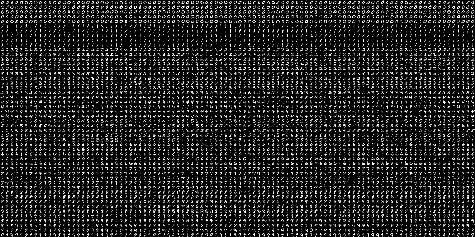
We are going to work with a very simple, small dataset of handwritten digits. The data is stored, in this case, in one image: digits.png, which is included in the Github repo (and shown here in Figure 1).
Figure 1: Dataset stored as an image
Image is 2000 pixels wide and 1000 pixels tall
It contains 5000 pixels, each one 20 pixels by 20 pixels in size
It has 500 images for each digit, organized into 5 20-pixel-tall rows
There are thus 50 20-pixel-tall rows
Data Wrangling
The first step in any machine learning task is data wrangling, or finding, storing, loading, and manipulating the data to be in the form that we need for the ML algorithm. We have to process the big image and break it up into the small images, attach the right label (0 through 9) to each image, and then convert the images so that they are one-dimensional arrays of floating-point numbers, 400-long, rather than 20 by 20. Then they will be suitable for training the KNearest algorithm.
Step 1: Break up the big picture
The code below reads in the digits image, converts it to grayscale, and then breaks it up into 20x20 chunks. The vsplit and hsplit functions from Numpy divide an array into the given number of sub-arrays: vsplit splits up the rows of the array, and hsplit splits up the columns. This code combines them using a list comprehension, producing a list of arrays of 20x20 grayscale images. The final step converts that list back into a Numpy array, with 50 rows, 100 columns, and each value within that is a small image.
sampleDataPath ="SampleData/"
digitDataIm = cv2.imread(sampleDataPath +"digits.png")# cv2.imshow("digit data image", digitDataIm)gray = cv2.cvtColor(digitDataIm, cv2.COLOR_BGR2GRAY)# Now we split the image first into 50 rows, and then each row into 100 columns, each 20x20 sizerows = np.vsplit(gray, 50)cells = [np.hsplit(row, 100) for row in rows]# Make it into a Numpy array: its size should be (50, 100, 20, 20)x = np.array(cells)# Make a matrix that is 50x100 and contains codes for each digit (0 through 9). These will be the targets, the labelsy = np.zeros((50, 100), np.float32)for digit inrange(10): row = digit *5 y[row:row+5, :] = digitprint(x.shape, y.shape)# Finally we will reshape the data to combine the 50 rows and 100 columns, to get something that is 5000 by 20 by 20x = x.reshape(-1, x.shape[2], x.shape[3])y = y.flatten()print(x.shape, y.shape)
Step 2: Divide data into training and validation sets
For this example, we will just have training data and validation data (we won’t break the dataset into three parts). We are going to use a function from the Scikit-Learn library. This is a great machine learning library for Python: it implements many ML tools, though typically not deep learning. Even when Python ML projects are not directly using Scikit-Learn, they may borrow tools from it. A common example is the train_test_split function in Scikit-Learn, which takes in the instances and target values for a dataset and divides them into training and validation (or testing) sets. It is remarkably useful: we’ll use it here to show how it works.
trainX, validX, trainY, validY = train_test_split(x, y,
                                                  train_size=0.75,
                                                  random_state=38271)
The first two inputs define the dataset: they must have the same size in the first dimension (5000 in our case).
The inputs to train_test_split are:
the input array, typically called X (required)
the target array, typically called Y (required)
train_size, the percentagee of the dataset to use for the training split, between 0.0 and 1.0 (optional)
random_state, a seed for the random number generator
The random seed makes sure that every time we run this function, we get the same division of data into training and validation (or testing) data. This is good if you want to compare the performance of different models on the same data: keeping the same split between training and validation ensures that the split itself won’t confound your results. It is especially important for deep learning, where we might need to train a model over several sessions: we need the same split every time.
Complete the KNN training and testing
The steps above end with data that is in the correct format for the KNearest object. Look back at the example that used artificial data, and follow that format to set up a KNearest object, and train it on the digits training data. Then, Call findNearest on the validX from above.
Compare the results array with the validY, which holds the correct values. Use that to compute the accuracy of the model.
Experiment!
After you get the KNN algorithm working on the data, try some experimentation.
A major component of working with machine learning is experimenting with how changing the parameters of the problem changes the outcomes. Try the experiments here, and be prepared to report on your findings!
Dig into the raw results a bit more. Compute the accuracy for each digit. Is KNN equally accurate on all categories, or does it do better on some than on others? Are there patterns to when it is right or wrong?
Try changing the number of neighbors. For which number of neighbors was the resulting accuracy the best?
Try changing the number of columns allocated to training versus testing. How does that affect the performance of the algorithm on the test data?
Convolutional Neural Networks
Simple convolutional neural networks are often used for classification or regression tasks. The convolutional/pooling section of the network finds useful patterns or features in an image, and then the dense neural network section uses the detected patterns/features to produce the right output.
For this task and the next one, we will write our programs in Google Colab, a free cloud-based environment designed for training deep learning models.
Using Google Colab
Google Colab allows you to create and run programs in the cloud. It makes it easy to work with complicated libraries like OpenCV, dlib, scikit-learn, and Tensorflow. You can also collaborate together with other people, and you have access to powerful cloud-based processors, both CPUs and GPUs.
Before starting this section, you should explore Google Colab (you have access through your Macalester email). You might look through these tutorials:
Share that notebook with your teammates, and with me
Work through the activity
Object Detection and Segmentation
Object detection models need to identify where interesting objects are, and then classify each object that has been found. They have more complex architectures than classification models, but they do often include convolutional/pooling sections. This activity will experiment with the YOLO (You Only Look Once) architecture, which has “backbone”, “neck”, and “head” sections. The first two sections do include convolutional/pooling layers.
Image segmentation goes a step further than object detection. Instead of finding bounding rectangles around objects of interest it marks each pixel in the image based on which object it belongs to. The output of this network is a copy of the image where each pixel has been market. YOLO provides a variation on its object detection model that performs segmentation instead.