This chapter will start by looking at some ways we can use existing trained models. It will then examine examples of machine learning for computer vision, starting from very simple data and models, and gradually increasing in complexity.

1 The Mediapipe library

The mediapipe library was created by Google to share models they developed and trained for a number of different computer vision tasks. We will examine several models that can detect faces, facial features, and hand and body positions (with an optional example of an object detection model).

To try these programs as you go along:

Join the ICA 16 Github assignment, and clone the repository onto your own computer
Download the MediapipeModels.zip file, unzip it, and move it into your project

The five starter programs are very similar to each other, because Mediapipe standardized the set-up and operation of models. What differs are the detected features returned by the model, and how we can visualize them by drawing them on the original image.

The five starter programs are all set up to work with the webcam: you may modify them to read a video file if you prefer. Each program:
- reads a frame from the video feed
- converts it to Mediapipe’s own image representation
- passes the result to the detector model, which returns an object that describes the items detected in the image (faces, hands, bodies)
- includes a TODO comment and a commented-out call to a function that would examine the detection results
- passes the detection results to a function that displays them on the original frame

1.1 Mediapipe face detection

Mediapipe has a state-of-the-art face detection model. Take a look at the Mediapipe Face Detection Guide for more details about the model itself.

The model detects a few specific landmarks of a face (eyes, nose tip, mouth, and sides of the face (cheeks or temples), and also provides a bounding box that surrounds the face. We will first walk through the demo program you have been provided, and then will look closely at the format of the data that is returned by the model.

If you can, open the mediapipeFaceDetect.py program, which is also included in the code block below.

The mediapipeFaceDetect.py program, demonstrates the face detection model and its results

"""
File: mediapipeFaceDetect.py
Date: Fall 2025

This program provides a demo showing how to use Mediapipe's simple face detection model, and to visualize the results.
"""

import math
import cv2

import mediapipe as mp
from mediapipe.tasks import python
from mediapipe.tasks.python import vision

MARGIN = 10  # pixels
ROW_SIZE = 10  # pixels
FONT_SIZE = 1
FONT_THICKNESS = 1
CIRCLE_COLOR = (0, 255, 0)  # green
TEXT_COLOR = (0, 255, 255)  # cyan, RGB, not a BGR


def runFaceDetect(source=0):
    """Main program, sets up the blaze face detection model and then runs it on a video feed."""

    # Set up model
    modelPath = "MediapipeModels/blaze_face_short_range.tflite"
    base_options = python.BaseOptions(model_asset_path=modelPath)
    options = vision.FaceDetectorOptions(base_options=base_options)
    detector = vision.FaceDetector.create_from_options(options)

    # Set up camera
    cap = cv2.VideoCapture(source)

    while True:
        gotIm, frame = cap.read()
        if not gotIm:
            break

        # Convert the frame to a Mediapipe image representation
        image = cv2.cvtColor(frame, cv2.COLOR_BGR2RGB)
        mp_image = mp.Image(image_format=mp.ImageFormat.SRGB, data=image)

        # Run the face detector model on the image
        detect_result = detector.detect(mp_image)

        # TODO: Uncomment this call to run the function that checks which way each detected face is pointing
        # findFacing(detect_result)

        annot_image = visualizeResults(mp_image.numpy_view(), detect_result)

        # Display the results on screen
        vis_image = cv2.cvtColor(annot_image, cv2.COLOR_RGB2BGR)
        cv2.imshow("Detected", vis_image)

        x = cv2.waitKey(10)                              
        if x > 0:
            if chr(x) == 'q':
                break
    cap.release()


def _normalized_to_pixel_coordinates(normalized_x, normalized_y, image_width, image_height):
    """Converts normalized value pair to pixel coordinates."""

    # Checks if the float value is between 0 and 1.
    def is_valid_normalized_value(value):
        return (value > 0 or math.isclose(0, value)) and (value < 1 or math.isclose(1, value))

    if not is_valid_normalized_value(normalized_x):
        normalized_x = max(0.0, min(1.0, normalized_x))
    if not is_valid_normalized_value(normalized_y):
        normalized_y = max(0.0, min(1.0, normalized_y))
    x_px = min(math.floor(normalized_x * image_width), image_width - 1)
    y_px = min(math.floor(normalized_y * image_height), image_height - 1)
    return x_px, y_px


def visualizeResults(image, detection_result):
    """Draws bounding boxes and keypoints on the input image and return it.
    Args:
        image: The input RGB image.
        detection_result: The list of all "Detection" entities to be visualized.
    Returns: Image with bounding boxes.
    """

    # Copy the original image and make changes to the copy
    annotated_image = image.copy()
    height, width, _ = image.shape

    for detection in detection_result.detections:
        # Draw bounding_box for each face detected
        bbox = detection.bounding_box
        start_point = bbox.origin_x, bbox.origin_y
        end_point = bbox.origin_x + bbox.width, bbox.origin_y + bbox.height
        cv2.rectangle(annotated_image, start_point, end_point, TEXT_COLOR, 3)

        # Draw face keypoints for each face detected
        for keypoint in detection.keypoints:
            keypoint_px = _normalized_to_pixel_coordinates(keypoint.x, keypoint.y, width, height)
            cv2.circle(annotated_image, keypoint_px, 3, CIRCLE_COLOR, -1)

        # Draw category label and confidence score as text on bounding box
        category = detection.categories[0]
        category_name = category.category_name
        category_name = '' if category_name is None else category_name
        probability = round(category.score, 2)
        result_text = category_name + ' (' + str(probability) + ')'
        text_location = (MARGIN + bbox.origin_x,
                         MARGIN + ROW_SIZE + bbox.origin_y)
        cv2.putText(annotated_image, result_text, text_location, cv2.FONT_HERSHEY_PLAIN,
                    FONT_SIZE, TEXT_COLOR, FONT_THICKNESS)

    return annotated_image


def findFacing(detect_results):
    """Takes in the face detection results and determines, for each face located, whether the
    face is pointing forward, to the left, or to the right. It prints a message with the results."""
    # TODO: for each face detected, determine the facing from the relative positions of each eye and
    # TODO: the edge of the face on that side
    pass


if __name__ == "__main__":
    runFaceDetect(0)

1: A set of constants that define the color, font, and other display details for visualizing the results
2: The main program
3: Set up the model (no need to understand the details)
4: Set up the video feed just as we have done
5: Convert the input frame to Mediapipe’s own representation of an image
6: Run the detector on the new representation of the frame
7: Call the helper function, for use with the ICA and homework
8: Call the visualizeResult function and show the final results
9: A function to convert from normalized coordinates to ordinary pixel coordinates for our image size
10: A function to draw the face results on the frame
11: A function to be completed by use for the ICA/Homework
12: The main script, which just calls the main function

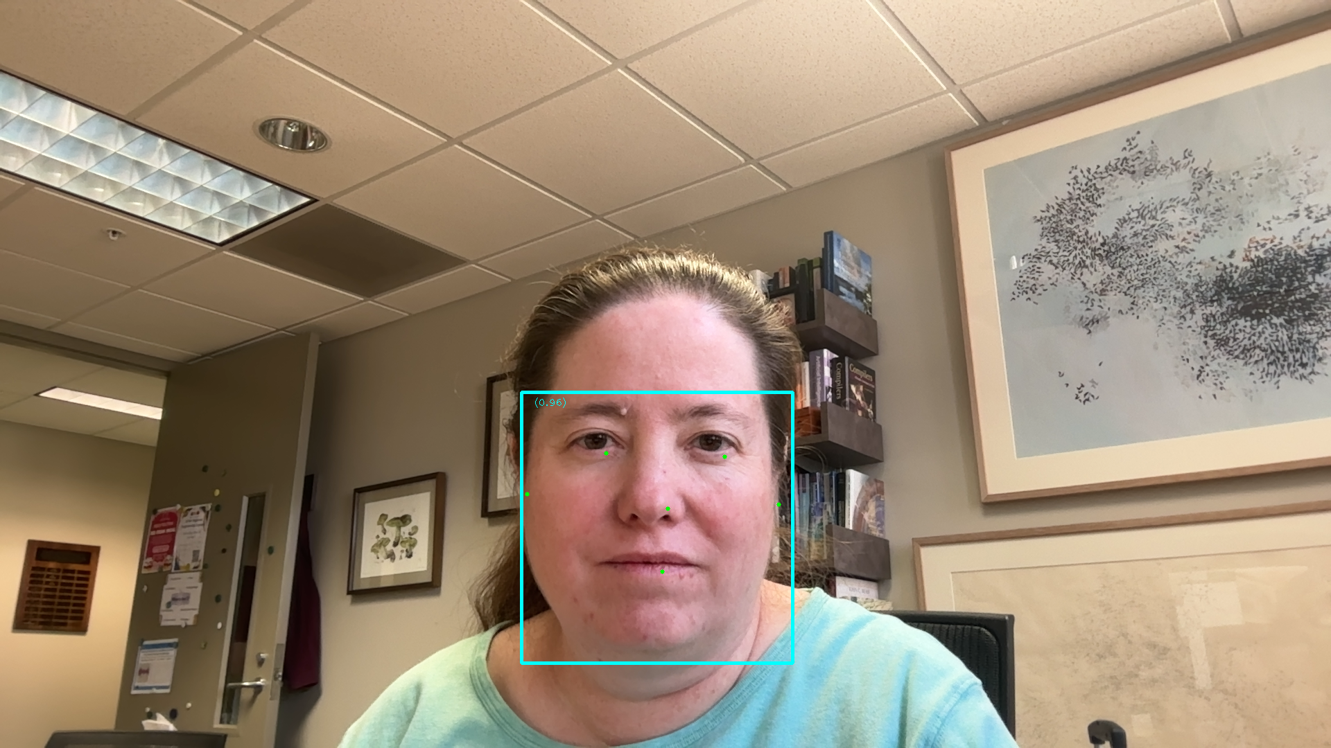
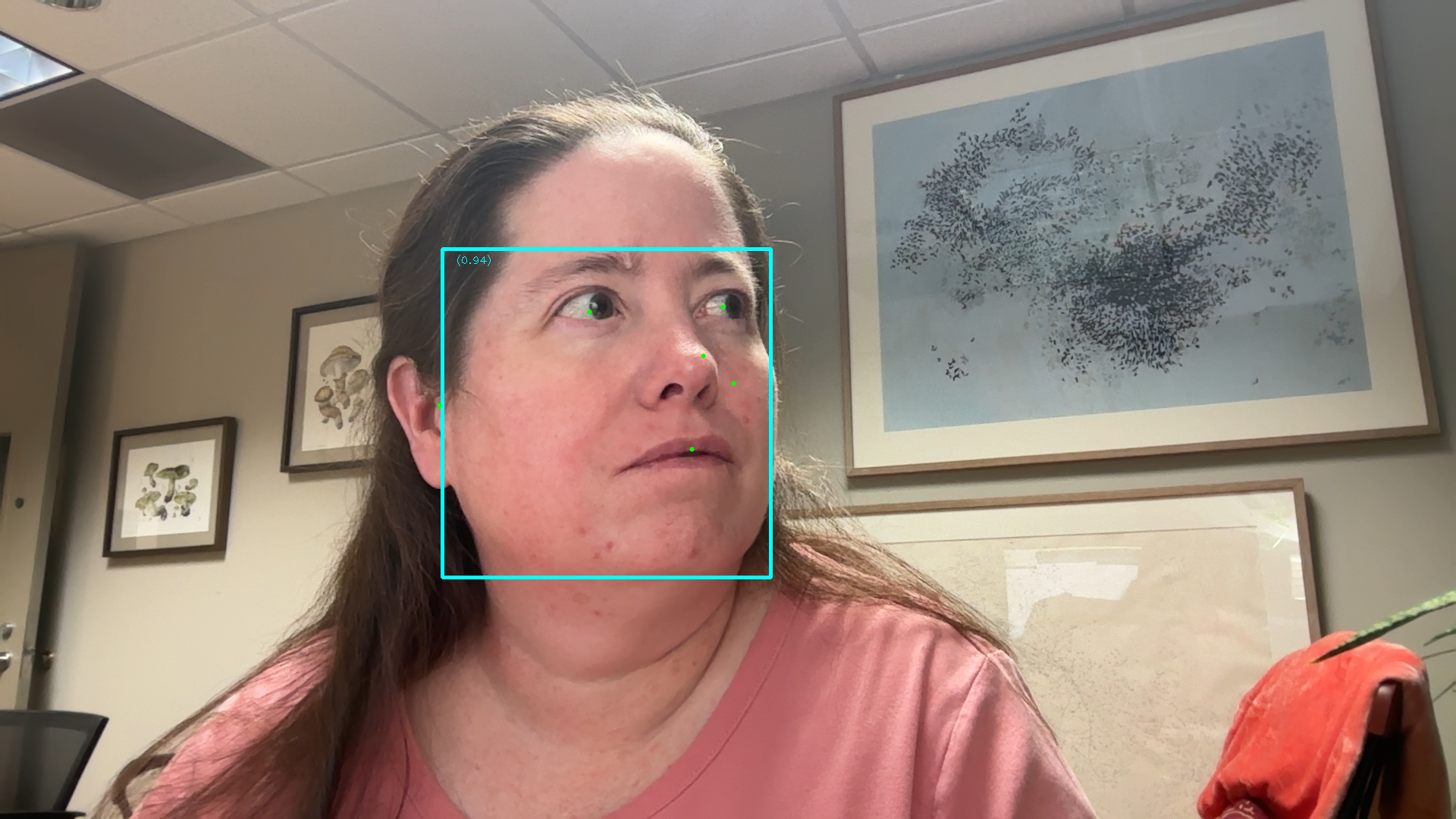
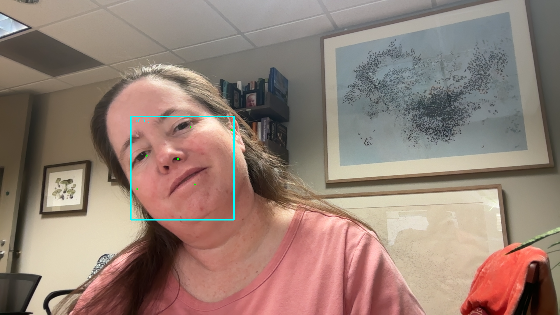
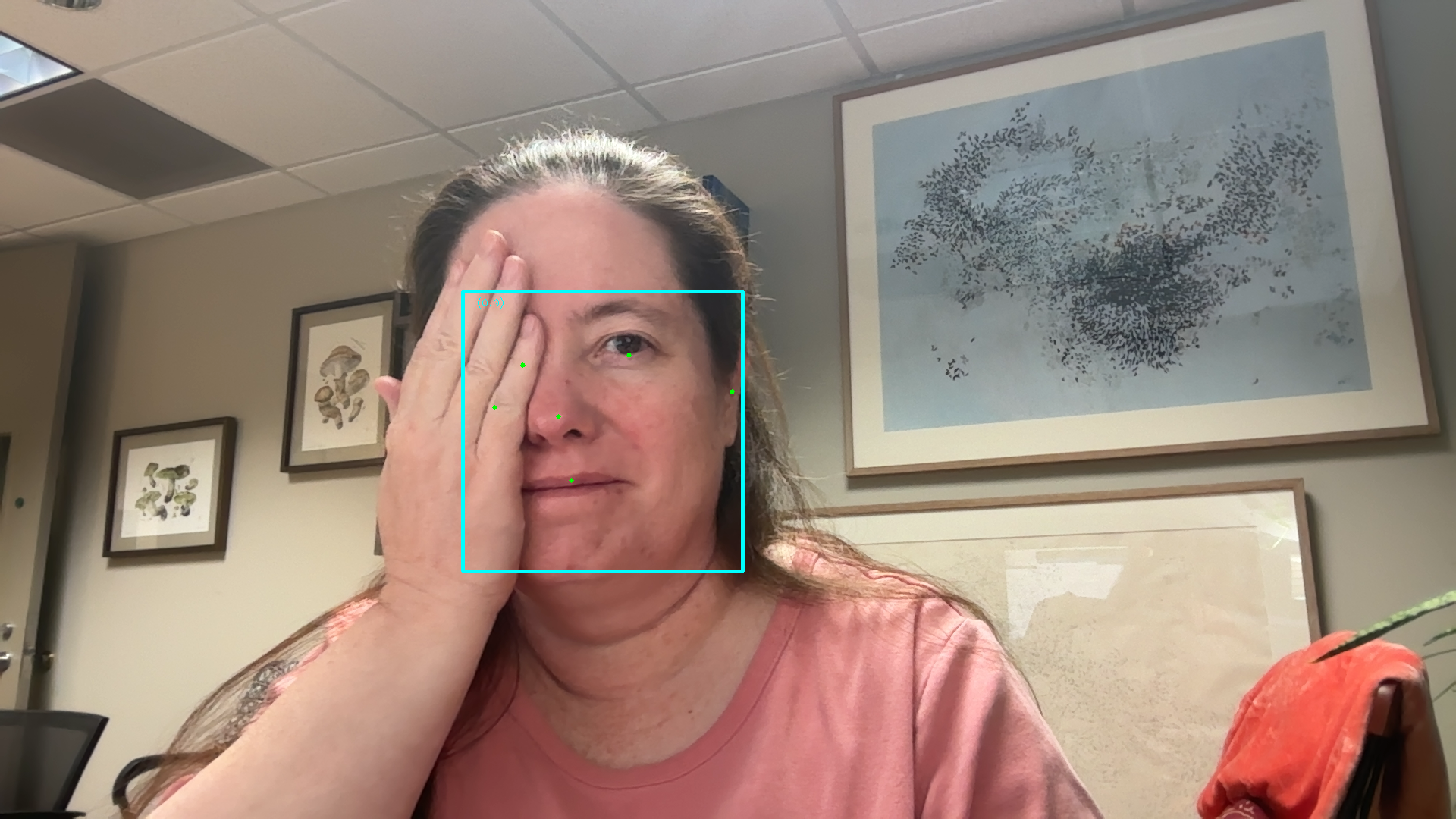
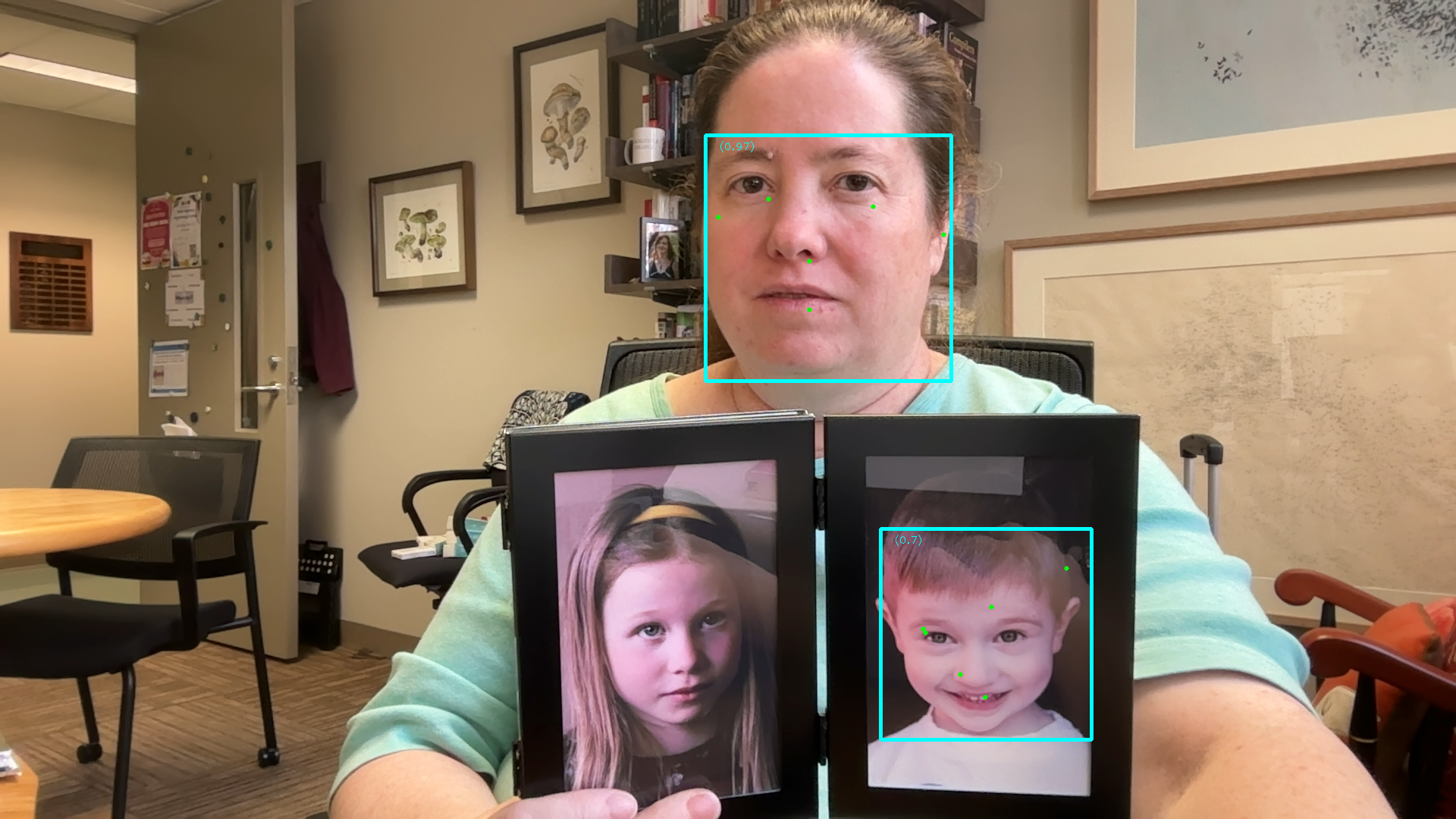
Figure 1 shows several screenshots from the running of this program. Notice that it can detect multiple faces, and each face detected includes several parts: a bounding rectangle, a confidence value, and six key points (eyes, nose, mouth, and cheeks/temples).

1.1.1 Examining the face detection program

There are four functions that make up this program, plus a very short script that calls the main function.

The runFaceDetect function is the main program. It loads the model, connects to the webcam, and then runs the model on frames from the webcam, displaying the results. It includes a call to an unfinished function that you could choose to implement for the in-class activity.

The visualizeResults function takes in an image represented as an RGB Numpy array (not quite OpenCV’s representation, but close), as well as the detection results from the model. It draws a bounding box around each face detected in the image, as well as several key points (eyes, nose, mouth, and edges of the face). It also adds a text label near the bounding box that lists the category (face) as well as the model’s confidence in its identification (probability that the identification is correct).

The _normalized_to_pixel_coordinates function is used to convert from the “normalized” coordinates the model produces to normal pixel coordinates. Normalized coordinates are scaled to be real numbers between 0.0 and 1.0, so they represent the proportion of the distance along the given dimension, while being independent of the actual width or height of the image (often images are resized to submit to a deep learning model). A normalized value of 0.0 would correspond to the leftmost column or topmost row in the image. A normalized value of 0.5 would be halfway across or down the image, and a normalized value of 1.0 would be the rightmost column or bottommost row.

The findFacing function does nothing initially, but is there for you to use when working with the detection results.

1.1.2 Face detection results

The results returned from the face detection model are complex and layered. The table below breaks down these results and how to access them.

Accessing results	Explanation
`dt = detector.detect(mp_image)`	`dt` is a `DetectionResult` object. It has one instance variable called `detections`
`dt.detections`	`detections` is a list containing `Detection` object, one for each face that has been detected. The list is empty when no faces are found
`detObj = dt.detections[0]`	`detObj` is a `Detection` object. It has three variables within it: `bounding_box`, `categories`, and `keypoints`
`bb = detObj.bounding_box` `bb.origin_x` `bb.origin_y` `bb.width` `bb.height`	`bounding_box` holds a `BoundingBox` object, which describes a rectangle. It has four values: `origin_x`, `origin_y`, `width` and `height`, in image pixel coordinates. They give the upper-left corner and width and height of a rectangle
`categs = detObj.categories`	`categs` is a list of `Category` objects, containing one category object
`cat1 = categs[0]` `conf = cat1.score`	`cat1` is a `Category` object. It has four variables in it: `index`, `score`, `display_name`, and `category_name`. We only need the score: the other three variables are used when detecting multiple kinds of objects, here we only have faces The score represents how confident the model is that it has found a face.
`kpts = detObj.keypoints`	`kpts` is a list containing six (x, y) coordinates. These points describe where certain landmarks on the face are detected to be.
`kpts[0]`	`kpts[0]` is a `NormalizedKeypoint` object, which has `x` and `y` variables, along with some others we don’t need. The coordinates are between 0.0 and 1.0.

The keypoints reported by this model are always in the same order:

kpts[0] is the eye that appears toward the left side of the image
kpts[1] is the eye that appears toward the right side of the image
kpts[2] is the nose
kpts[3] is the mouth
kpts[4] is the ear that appears toward the left side of the image
kpts[5] is the ear that apepars toward the right side of the image

In the ICA code, there is a text file, faceDetectResults.txt that shows the structure of the results for zero faces, one face, and two faces detected.

1.2 Facial feature detection

We can go well beyond finding a handful of keypoints on a face. Mediapipe includes a more elaborate face landmark detection object. Look at the Mediapipe Face Landmark Detection guide for more details.

The face landmarker actually runs three separate models on the image it is given:

The face detection model from the previous section
A model that detects nearly 500 face landmarks
A model that identifies blendshapes: configurations of the face landmarks that indicate a particular higher-level pattern, such as “outer end of left eyebrow raised”

With the outputs from these models, we should be able to identify general emotions expressed in a face, or use these landmarks for motion capture, or to augment the user’s face with fake glasses, flowers, or makeup.

If you can, open the mediapipeFaceLandmark.py program, which is also included in the code block below.

The mediapipeFaceLandmark.py program, demonstrates the facial landmark models and their results

"""
File: mediapipeFaceLandmark.py
Date: Fall 2025

This program provides a demo showing how to use Mediapipe's facial landmark model, and to visualize the results.
"""

import cv2
import numpy as np

import mediapipe as mp
from mediapipe.tasks import python
from mediapipe.tasks.python import vision

from mediapipe import solutions
from mediapipe.framework.formats import landmark_pb2
import matplotlib.pyplot as plt


def runFacialLandmarks(source=0):
    # Set up model
    modelPath = "MediapipeModels/face_landmarker_v2_with_blendshapes.task"
    base_options = python.BaseOptions(model_asset_path=modelPath)
    options = vision.FaceLandmarkerOptions(base_options=base_options,
                                           output_face_blendshapes=True,
                                           output_facial_transformation_matrixes=True,
                                           num_faces=1)
    detector = vision.FaceLandmarker.create_from_options(options)

    # Set up camera
    cap = cv2.VideoCapture(source)

    while True:
        gotIm, frame = cap.read()
        if not gotIm:
            break

        # Convert image to Mediapipe image format
        image = cv2.cvtColor(frame, cv2.COLOR_BGR2RGB)
        mp_image = mp.Image(image_format=mp.ImageFormat.SRGB, data=image)

        # Run facial landmark detector
        detect_result = detector.detect(mp_image)

        # TODO: Uncomment this call to run the function that checks whether eyes are open or closed
        # findEyes(detect_result)

        annot_image = visualizeResults(mp_image.numpy_view(), detect_result)
        vis_image = cv2.cvtColor(annot_image, cv2.COLOR_RGB2BGR)
        cv2.imshow("Detected", vis_image)

        x = cv2.waitKey(10)
        if x > 0:
            if chr(x) == 'q':
                break
            elif chr(x) == 'b':
                plot_face_blendshapes_bar_graph(detect_result.face_blendshapes[0])
    cap.release()


def visualizeResults(rgb_image, detection_result):
    """
    Draw the face landmark mesh onto a copy of the input RGB image and returns it
    :param rgb_image: an image in RGB format (as a Numpy array)
    :param detection_result: The results of running the face landmarker model
    :return: a copy of rgb_image with face landmark mesh drawn on it
    """
    annotated_image = np.copy(rgb_image)
    face_landmarks_list = detection_result.face_landmarks

    # Loop through the detected faces to visualize.
    for idx in range(len(face_landmarks_list)):
        face_landmarks = face_landmarks_list[idx]

        # Draw the face landmarks.
        face_landmarks_proto = landmark_pb2.NormalizedLandmarkList()
        face_landmarks_proto.landmark.extend([
            landmark_pb2.NormalizedLandmark(x=landmark.x, y=landmark.y, z=landmark.z) for landmark in face_landmarks
        ])

        solutions.drawing_utils.draw_landmarks(
            image=annotated_image,
            landmark_list=face_landmarks_proto,
            connections=mp.solutions.face_mesh.FACEMESH_TESSELATION,
            landmark_drawing_spec=None,
            connection_drawing_spec=mp.solutions.drawing_styles
            .get_default_face_mesh_tesselation_style())
        solutions.drawing_utils.draw_landmarks(
            image=annotated_image,
            landmark_list=face_landmarks_proto,
            connections=mp.solutions.face_mesh.FACEMESH_CONTOURS,
            landmark_drawing_spec=None,
            connection_drawing_spec=mp.solutions.drawing_styles
            .get_default_face_mesh_contours_style())
        solutions.drawing_utils.draw_landmarks(
            image=annotated_image,
            landmark_list=face_landmarks_proto,
            connections=mp.solutions.face_mesh.FACEMESH_IRISES,
            landmark_drawing_spec=None,
            connection_drawing_spec=mp.solutions.drawing_styles
            .get_default_face_mesh_iris_connections_style())

    return annotated_image


def plot_face_blendshapes_bar_graph(face_blendshapes):
    """
    Creates a plt bar graph to show how much each blendshape is present in a given image
    :param face_blendshapes: output from the blendshapes model
    :return:
    """
    # Extract the face blendshapes category names and scores.
    face_blsh_names = [face_blsh_category.category_name for face_blsh_category in face_blendshapes]
    face_blsh_scores = [face_blsh_category.score for face_blsh_category in face_blendshapes]
    # The blendshapes are ordered in decreasing score value.
    face_blsh_ranks = range(len(face_blsh_names))

    fig, ax = plt.subplots(figsize=(12, 12))
    bar = ax.barh(face_blsh_ranks, face_blsh_scores, label=[str(x) for x in face_blsh_ranks])
    ax.set_yticks(face_blsh_ranks, face_blsh_names)
    ax.invert_yaxis()

    # Label each bar with values
    for score, patch in zip(face_blsh_scores, bar.patches):
        plt.text(patch.get_x() + patch.get_width(), patch.get_y(), f"{score:.4f}", va="top")

    ax.set_xlabel('Score')
    ax.set_title("Face Blendshapes")
    plt.tight_layout()
    plt.show()


def findEyes(detect_result):
    """Takes in the facial landmark results and determines, for each face located, whether the
        eyes are open or closed. Print a message"""
    # TODO: Look at the blendshapes for the eyes and determine if the eyes are open or closed
    pass


if __name__ == "__main__":
    runFacialLandmarks(0)

1: Set up the model; note the num_faces input limits how many faces it will detect and you can change it
2: Set up the camera as usual
3: Convert the camera frame to a Mediapipe image
4: Run the face landmark detector on the converted image
5: Call optional function that processes the results for the ICA
6: Draw a visualization of the results on the frame
7: Function that draws results on the frame
8: Functino that displays what blendshapes were found
9: Function for processing the detected results for the ICA
10: Main script that just calls runFacialLandmarks

Face landmarks are defined as 3-d points, with x and y values defined as usual in terms of the image itself, but also including distance in the z axis, which is perpendicular to both x and y, running between the camera and the camera’s subjects. The origin for x and y are in the upper left corner of the image, the origin for the z axis lies where the main face sits in the image. The z axis has to be inferred from the size of the face, based on the training data the model was trained on, so it is often much less accurate than the x and y coordinates.

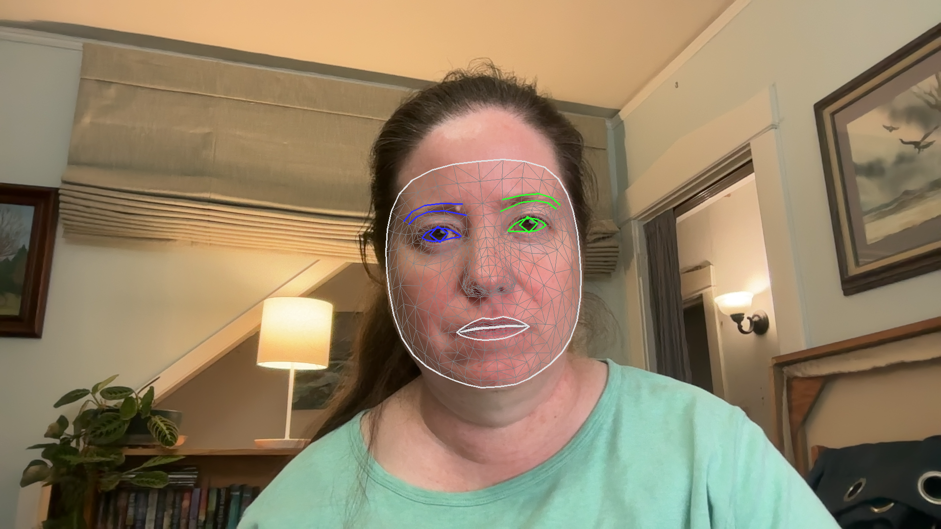
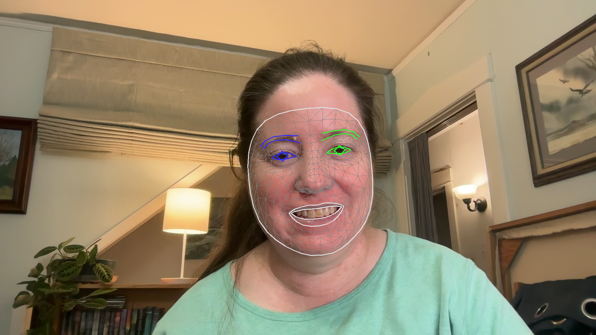
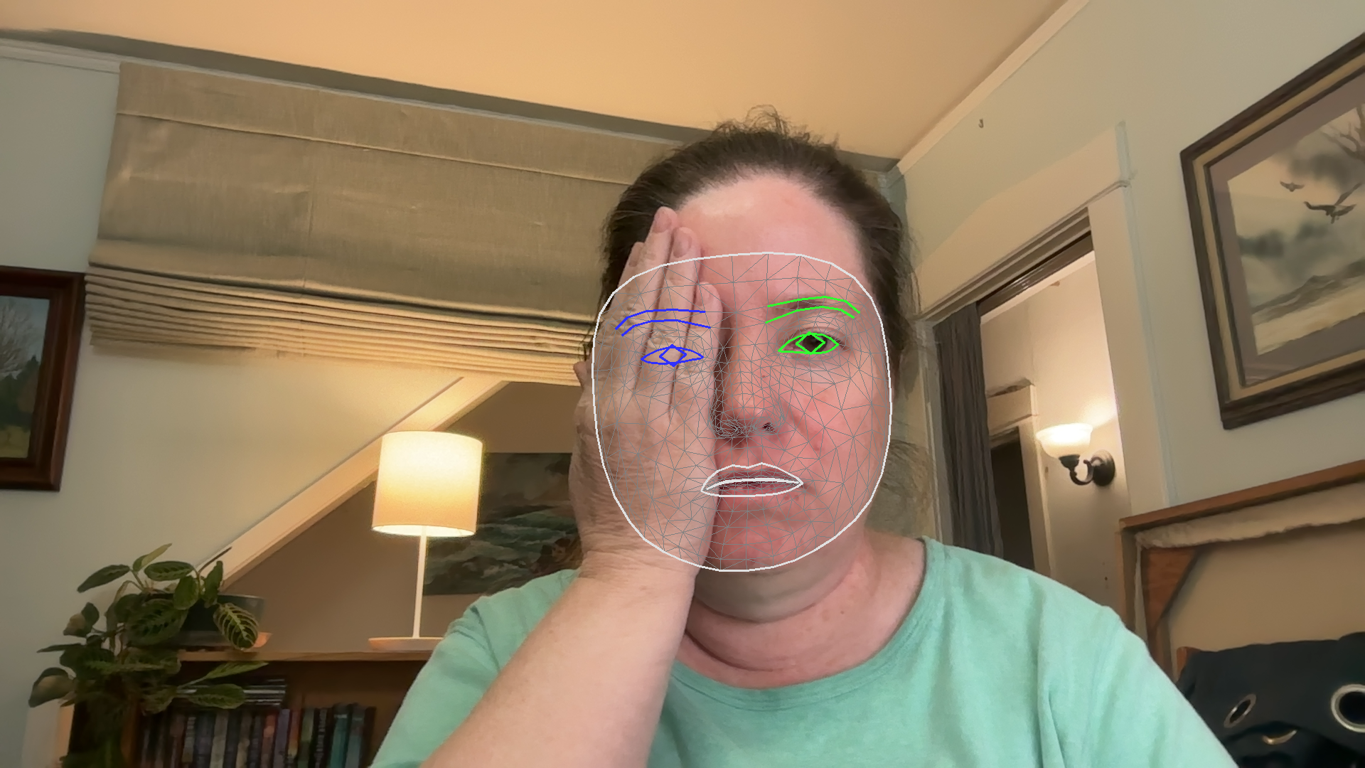
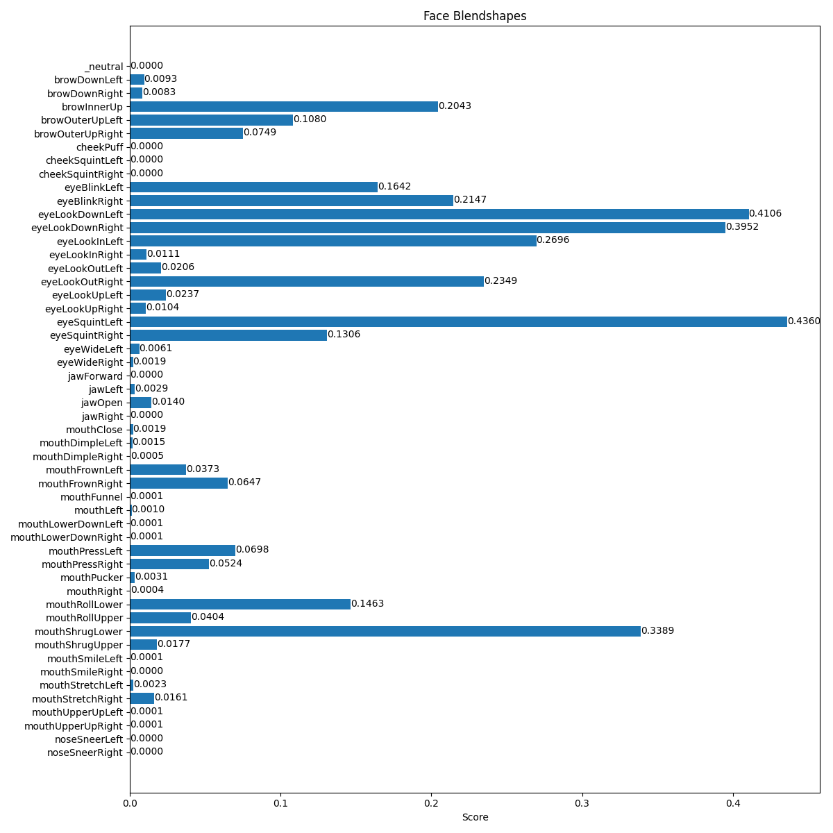
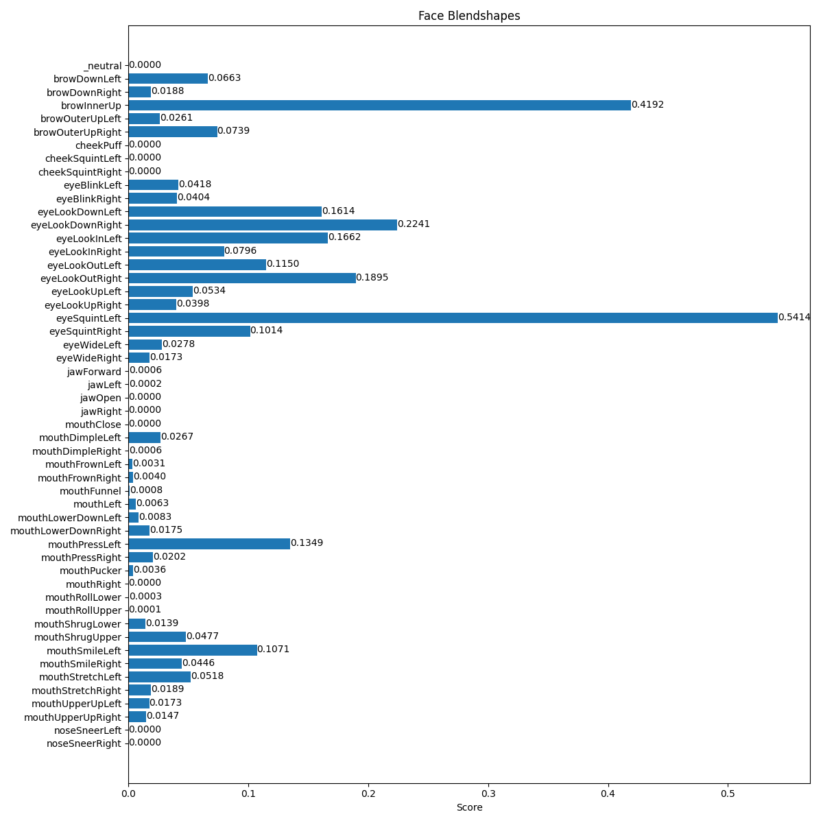
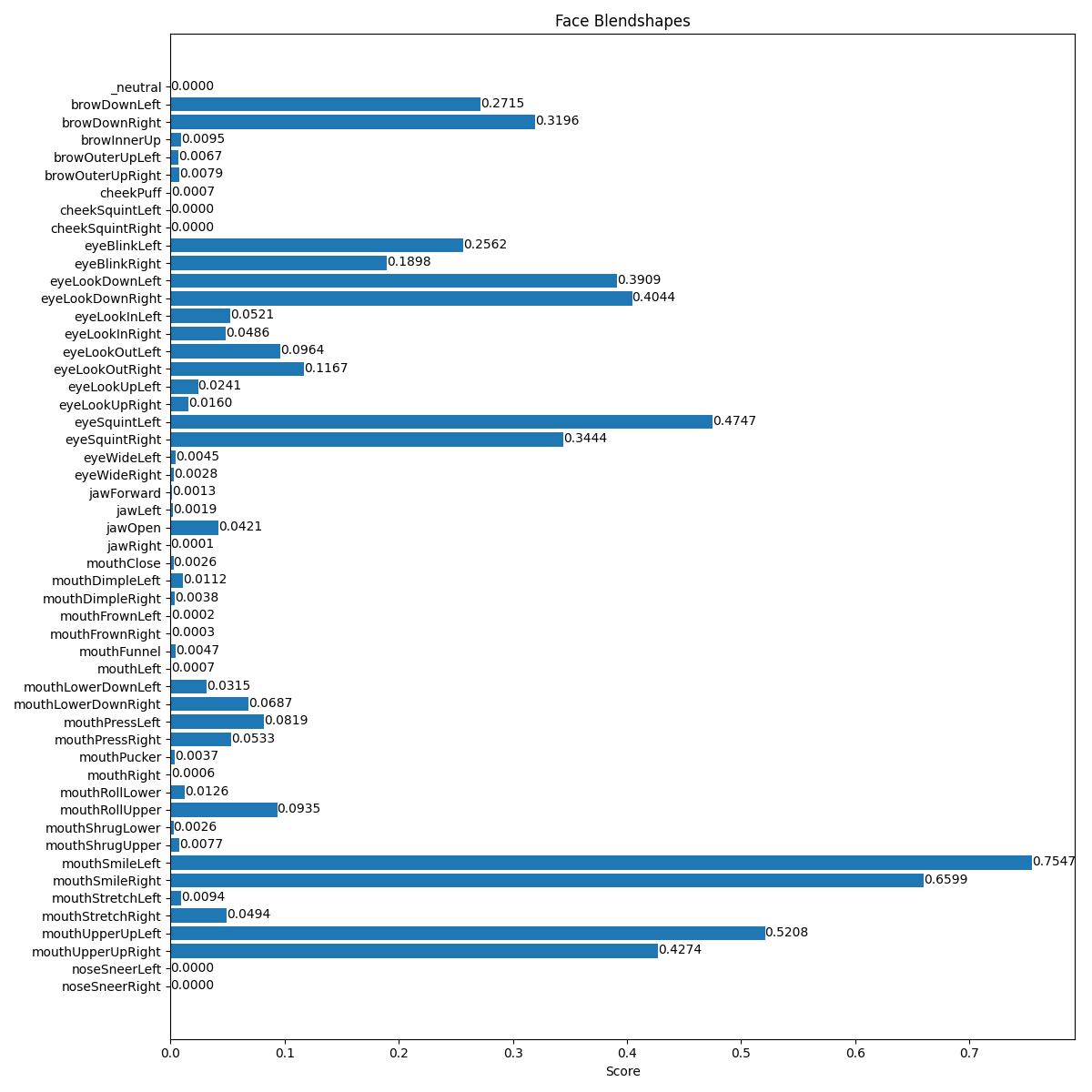
There are more than 400 landmarks found by this model (see the detailed image provided on the Mediapipe website)

Figure 2 shows several screenshots from the running of this program, and Figure 3 shows the blendshapes information that goes along with some of them.

1.2.1 Examining the facial landmark detection program

Much like the previous program, this program has four functions.

The runFacialLandmarks function is the main program, setting up the facial landmark detector and then looping over the frames of a video feed, and running the detector on each frame.

The visualizeResults function maps the 3d coordinates onto the 3d image, and draws an outline around the borders of the face, as well as outlining the mouth and eyes. It even identifies the center of the eye with a diamond. Notice that this code calls Mediapipe drawing tools because of the complexity of what is being drawn.

The plot_face_blendshapes_bar_graph function is a somewhat glitchy function for building a matplotlib bar graph that shows how strongly each blendshape appears in the current frame. The program had a tendency to crash after creating this bar graph, so use it sparingly.

The findEyes function will be completed as a part of the ICA, if you choose this portion. It will determine if eyes are open or shut.

1.2.2 Face landmark results

The results returned from the face landmark detector, while long, have less complex structure than some of the other programs. The table below shows how to access each part of the results, and what each part means.

Accessing results	Explanation
`dt = detector.detect(mp_image)`	`dt` is a `FaceLandmarkerResult` object. It has three variables within it: `face_landmarks`, `face_blendshapes`, and `facial_transformation_matrixes`. We might use the landmarks themselves and the blendshapes, not the matrixes
`dt.face_landmarks`	`face_landmarks` is a list of lists. Each sublist corresponds to one face that has been detected.
`lmarks = dt.face_landmarks[0]`	`lmarks` is a list of normalized coordinates, one for each facial landmark detected. Each coordinate is a `NormalizedLandmark` object.
`lmarks[0]`	`lmarks[0]` is one `NormalizedLandmark`, which has `x`, `y`, and `z` variables, along with some others we don’t need. Each `x`, `y`, and `z` values is in the range from 0.0 to 1.0
`blshList = dt.face_blendshapes`	`blshList` is a list of is a lists of `Category` objects. Each sublist corresponds to one of the faces detected: the length of the `face_landmarks` list and `blshList` are the
`blsh1 = blshList[0]`	`blsh1` is a list of 52 `Category` objects, one for each of the blendshapes that have been learned (see list below).
`cat1 = blsh1[0]` `cat1.index` `cat1.score` `cat1.category_name`	`cat1` is a `Category` object (specifically the `neutral` blendshape). This is the same type of object used by the face detector for the face score. Here, we do want to use three of the four variables: `index`, `score`, and `category_name`. The index tells us which blendshape it is, the `score` represents how strongly that blendshape is present, and `category_name` is a printable label for which blendshape.

In the ICA code, there is a text file, faceLandmarkResults.txt that shows the structure of the results for zero faces, one face, and two faces detected.

1.2.3 Blendshapes

Each blendshape combines sets of landmarks and their relative positions to identify larger-scale movements of parts of the face. The blendshape model was trained on the landmark data to predict the correct blendshapes shown. These are not emotions, and not even facial expressions. But they could be the building blocks for identifying facial expressions. The table below lists the names of the 52 blendshapes that can be identified.

Blendshapes	Blendshapes	Blendshapes	Blendshapes
0 - neutral	14 - eyeLookInRight	27 - mouthClose	40 - mouthRollLower
1 - browDownLeft	15 - eyeLookOutLeft	28 - mouthDimpleLeft	41 - mouthRollUpper
2 - browDownRight	16 - eyeLookOutRight	29 - mouthDimpleRight	42 - mouthShrugLower
3 - browInnerUp	17 - eyeLookUpLeft	30 - mouthFrownLeft	43 - mouthShrugUpper
4 - browOuterUpLeft	18 - eyeLookUpRight	31 - mouthFrownRight	44 - mouthSmileLeft
5 - browOuterUpRight	19 - eyeSquintLeft	32 - mouthFunnel	45 - mouthSmileRight
6 - cheekPuff	20 - eyeSquintRight	33 - mouthLeft	46 - mouthStretchLeft
7 - cheekSquintLeft	21 - eyeWideLeft	34 - mouthLowerDownLeft	47 - mouthStretchRight
8 - cheekSquintRight	22 - eyeWideRight	35 - mouthLowerDownRight	48 - mouthUpperUpLeft
9 - eyeBlinkLeft	23 - jawForward	36 - mouthPressLeft	49 - mouthUpperUpRight
10 - eyeBlinkRight	24 - jawLeft	37 - mouthPressRight	50 - noseSneerLeft
11 - eyeLookDownLeft	25 - jawOpen	38 - mouthPucker	51 - noseSneerRight
12 - eyeLookDownRight	26 - jawRight	39 - mouthRight	52 - tongueOut
13 - eyeLookInLeft

1.3 Hand landmark skeletons

In this section we will examine how to use Mediapipe’s hand landmark detector. This detects landmarks on a hand, and creates a skeleton of landmarks: it connects certain landmarks together as they correspond to connected body parts, allowing us to draw a skeleton-like framework showing how landmarks naturally fit together. It can detect whether a given skeleton is a right or left hand. See the Mediapipe Hand Landmarks Detection Guide for more details.

The detector actually integrates two separate models: a palm detector and a hand landmark detector that uses the palm location to simplify its task.

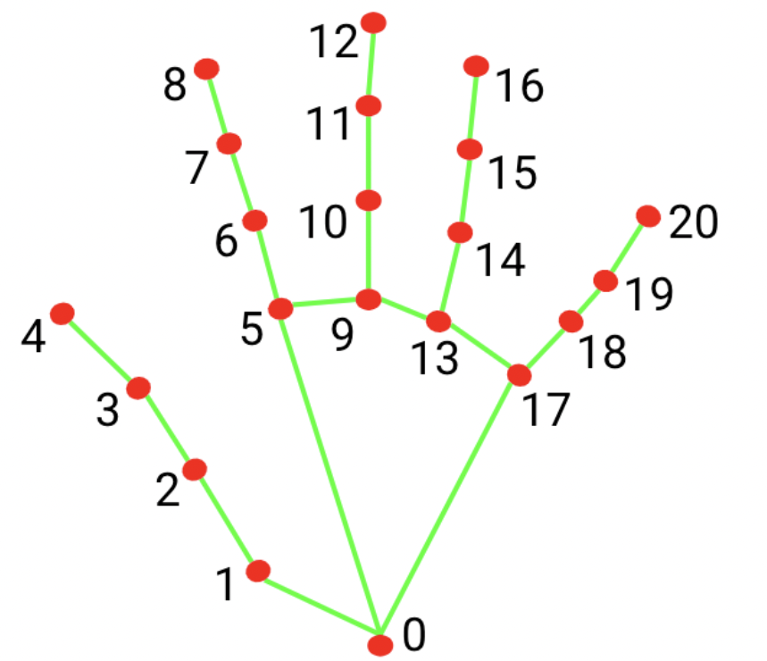
There are 21 hand landmarks for each hand. Figure 4, from the Mediapipe guide, illustrates what all 21 landmarks represent:

If you can, open the mediapipeHand.py program, which is also included in the code block below.

The mediapipeHand.py program, demonstrates the hand landmark detection model and its results

"""
File: mediapipeHand.py
Date: Fall 2025

This program provides a demo showing how to use Mediapipe's hand pose detection model, and how to visualize
the results.
"""

import cv2
import numpy as np

import mediapipe as mp
from mediapipe.tasks import python
from mediapipe.tasks.python import vision

from mediapipe import solutions
from mediapipe.framework.formats import landmark_pb2

MARGIN = 10  # pixels
FONT_SIZE = 1
FONT_THICKNESS = 1
HANDEDNESS_TEXT_COLOR = (88, 205, 54)  # vibrant green


def runHandModel(source):
    """Main program, sets up the model, then runs it on a video feed"""

    # Set up model
    modelPath = "MediapipeModels/hand_landmarker.task"
    base_options = python.BaseOptions(model_asset_path=modelPath)
    options = vision.HandLandmarkerOptions(base_options=base_options, num_hands=2)
    detector = vision.HandLandmarker.create_from_options(options)

    # Set up camera
    cap = cv2.VideoCapture(source)

    while True:
        ret, frame = cap.read()
        if not ret:
            break

        # Convert camera image to Mediapipe representation
        image = cv2.cvtColor(frame, cv2.COLOR_BGR2RGB)
        mp_image = mp.Image(image_format=mp.ImageFormat.SRGB, data=image)

        # Run the hand pose detector, receive detection information
        detect_result = detector.detect(mp_image)

        # TODO: Uncomment this to detect whether the hand is open palm or fist
        # findHandPose(detect_result)

        # Draw the results using mediapipe tools, then display the result
        annot_image = visualizeResults(mp_image.numpy_view(), detect_result)
        vis_image = cv2.cvtColor(annot_image, cv2.COLOR_RGB2BGR)
        cv2.imshow("Detected", vis_image)

        x = cv2.waitKey(10)
        if x > 0:
            if chr(x) == 'q':
                break
    cap.release()


def visualizeResults(rgb_image, detection_result):
    """
    Draws hand skeleton for each hand visible in an image
    :param rgb_image: An RGB image array
    :param detection_result: The results from the hand landmark detector
    :return: a copy of the input array with the hand skeleton drawn on it, labeled with left or right handedness
    """
    annotated_image = np.copy(rgb_image)

    hand_landmarks_list = detection_result.hand_landmarks
    handedness_list = detection_result.handedness

    # Loop through the detected hands to visualize.
    for idx in range(len(hand_landmarks_list)):
        hand_landmarks = hand_landmarks_list[idx]
        handedness = handedness_list[idx]

        # Draw the hand landmarks.
        hand_landmarks_proto = landmark_pb2.NormalizedLandmarkList()
        hand_landmarks_proto.landmark.extend([
            landmark_pb2.NormalizedLandmark(x=landmark.x, y=landmark.y, z=landmark.z) for landmark in hand_landmarks
        ])
        solutions.drawing_utils.draw_landmarks(
            annotated_image,
            hand_landmarks_proto,
            solutions.hands.HAND_CONNECTIONS,
            solutions.drawing_styles.get_default_hand_landmarks_style(),
            solutions.drawing_styles.get_default_hand_connections_style())

        # Get the top left corner of the detected hand's bounding box.
        height, width, _ = annotated_image.shape
        x_coordinates = [landmark.x for landmark in hand_landmarks]
        y_coordinates = [landmark.y for landmark in hand_landmarks]
        text_x = int(min(x_coordinates) * width)
        text_y = int(min(y_coordinates) * height) - MARGIN

        # Draw handedness (left or right hand) on the image.
        cv2.putText(annotated_image, f"{handedness[0].category_name}",
                    (text_x, text_y), cv2.FONT_HERSHEY_DUPLEX,
                    FONT_SIZE, HANDEDNESS_TEXT_COLOR, FONT_THICKNESS, cv2.LINE_AA)

    return annotated_image


def findHandPose(detect_results):
    """Takes in the hand position results and determines whether the hand is an open palm, fingers up,
    or a closed fist"""
    # TODO: for each detected hand, extract the appropriate features and check them. Print the result
    pass


if __name__ == "__main__":
    runHandModel(0)

1: Set up the hand landmark model; note that we can specify the maximum number of hands for it to recognize
2: Convert the video frame to a Mediapipe image
3: Run the model on the converted image
4: Call an optional function to process the results
5: Draw the results on the frame, and display it
6: A function to draw the results
7: A function for you to complete with the ICA
8: The main script that calls the main function

Much like face landmarks, the hand landmarks are defined as 3d points, with the z axis perpendicular to the x and y axes, along the line between camera and camera subject. The origin for the z axis is typically one of the landmarks, such as the base of the palm.

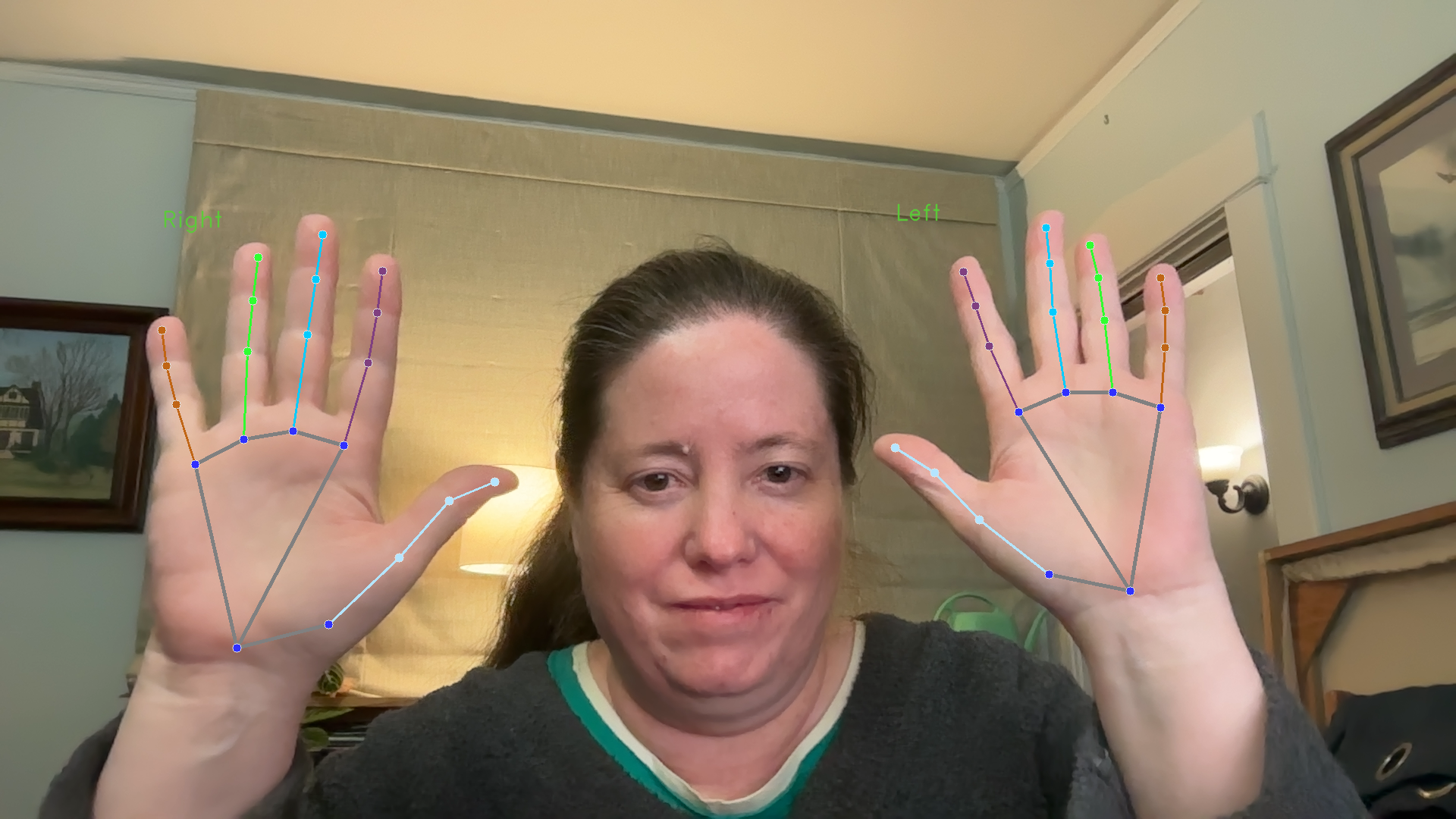
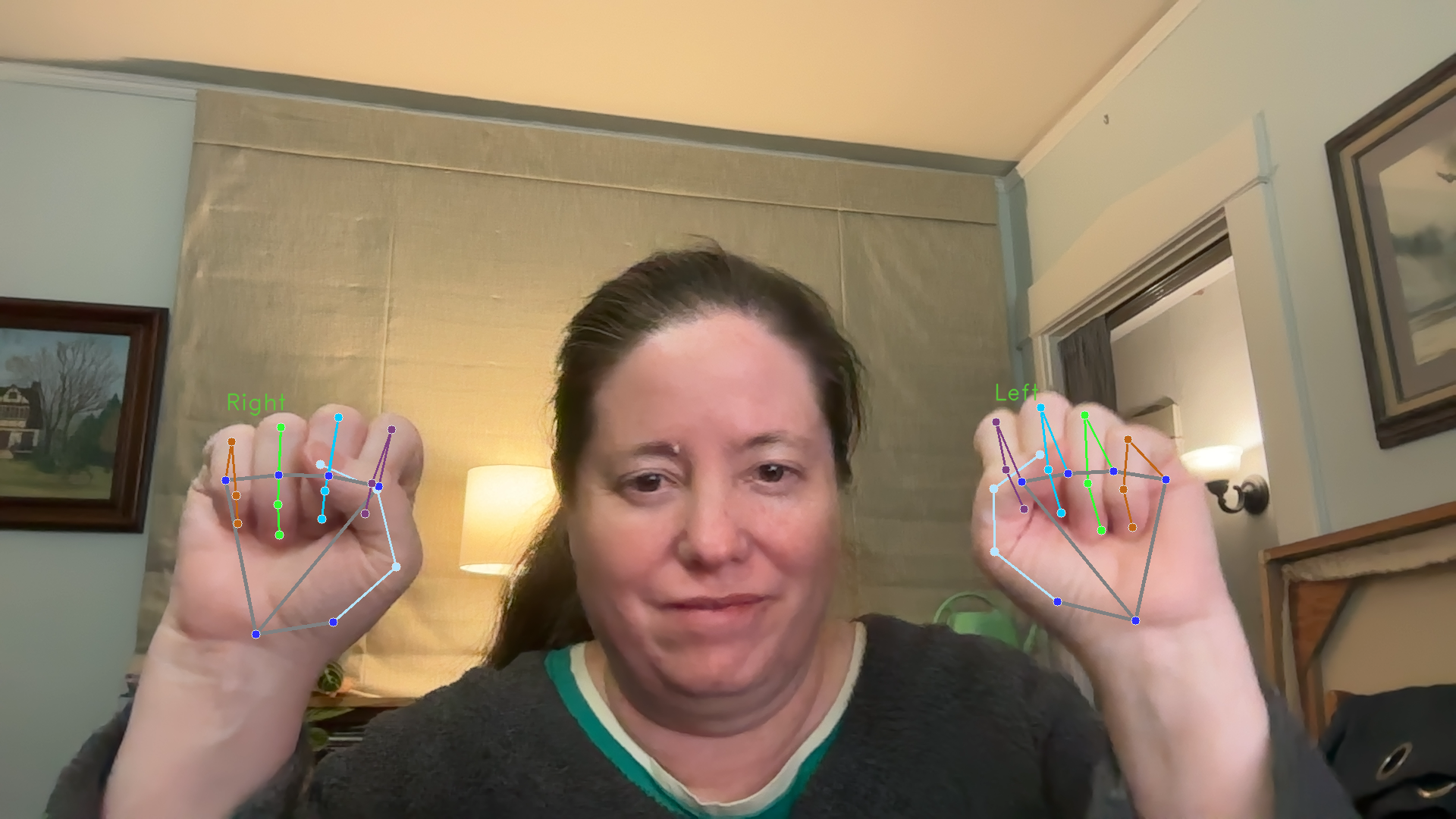
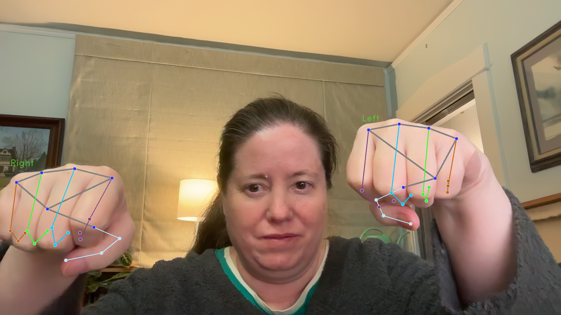
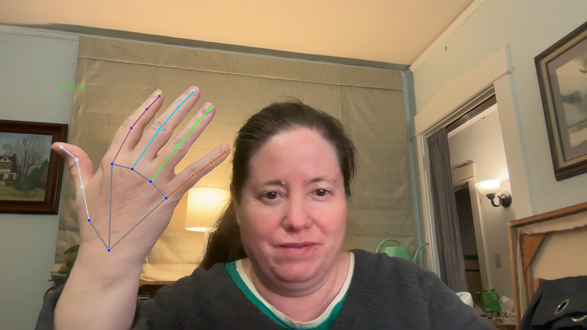
Figure 5 shows several screenshots from the running of this program, showing one or both hands in various orientations. Pay attention to the skeleton form, which allows us to estimate the location of landmarks that are blocked from view.

1.3.1 Examining the hand landmark detection program

This program has three functions, plus a short main script that calls the main function.

The runHandMode function is the main function. Like the other demo programs, it sets up the hand landmark model and then uses it on frames from a video feed. It includes a commented-out function that can interpret the results from the model, if you choose to work on this program.

The visualizeResults function draws the results on the current frame. It uses Mediapipe’s more sophisticated drawing tools, in order to draw the skeleton and the 3d points most easily.

The findHandPose function is for you to implement, if you choose. It would try to distinguish between open palms and fists.

1.3.2 Hand landmark results

The results returned from the hand landmark detector have many fewer landmarks than the facial landmark detector. That said, it includes each hand landmark in two forms, as a NormalizedLandmark and as a “world landmark,” where the values are given as distances in metric units. The table below shows how to access each part of the results, and what each part means.

Accessing results	Explanation
`dt = detector.detect(mp_image)`	`dt` is a `HandLandmarkerResult` object. It has three variables within it: `handedness`, `hand_landmarks`, and `hand_world_landmarks`. We could use any of these three, although the world landmarks are unreliable below a certain confidence score.
`dt.handedness`	`handedness` is a list of lists. Each sublist corresponds to one hand that has been detected.
`catList = dt.handedness[0]` * `catList[0].index` * `catList[0].score` * `catList[0].category_name`	`catList` is a list containing a `Category` object. Here the `index` variable tells us right vs. left hand, the `score` variable holds the confidence, and the `category_name` holds a string version of which hand.
`hlmarks = dt.hand_landmarks`	`hlmarks` is a list of lists. Each sublist corresponds to one hand that has been detected. Each set of data puts the data for the same hand in the same position in the list.
`landList = hlmarks[0]`	`landList` is a list of `NormalizedLandmark` objects, one for each landmark. As in other examples, each landmark object has `x`, `y`, and `z` variables, with `x` and `y` values scaled to be between 0.0 and 1.0
`wldmarks = dt.world_hand_landmarks`	`wldmarks` has the same structure as `hlmarks` above. The The difference is that the 3d points are represented as `Landmark` objects, with values in global measurements, some kind of metric unit here. For hands, probably centimeters.

In the ICA code, there is a text file, handLandmarkResults.txt that shows the structure of the results for no hands, one hand, two hands, and four hands (in an abbreviated form).

1.4 Mediapipe pose landmark skeletons

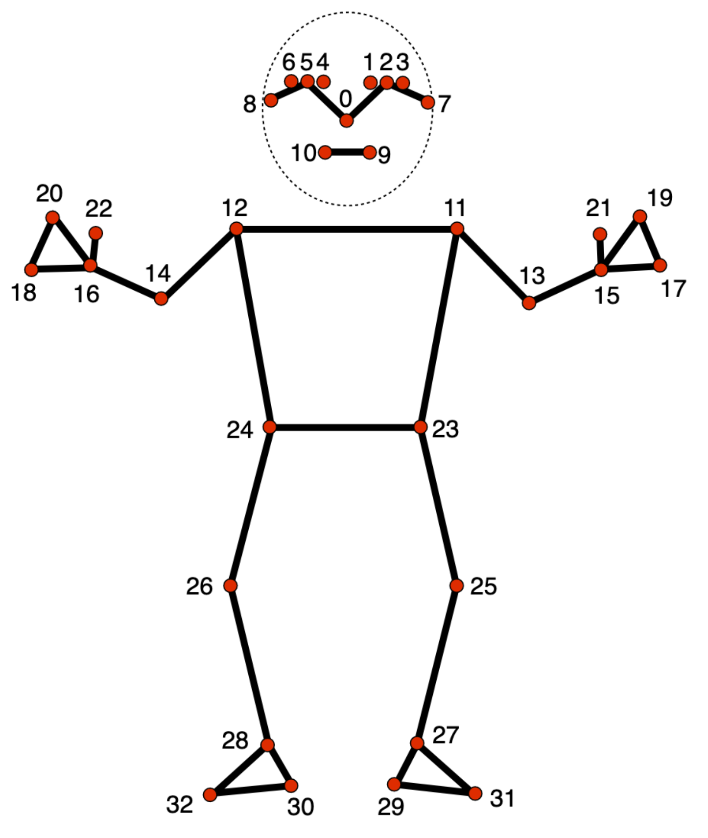
Mediapipe’s pose landmark detector finds landmarks on a whole body (or as much as is visible to the camera), and creates a skeleton view of the landmarks and how they connect to each other. The detector tracks 33 landmarks of the body. See the Mediapipe PoseLandmarks Detection Guide for more details.

Much like other landmarks, the pose skeleton points are defined as 3d points, with the z axis used for the dimension between camera and subjects. There are 33 body pose landmarks. Figure 6, from the Mediapipe guide, illustrates what all 33 landmarks represent:

If you can, open the mediapipePose.py program, which is also included in the code block below.

The mediapipePose.py program, demonstrates the body pose landmark detection model and its results

"""
File: mediapipePose.py
Date: Fall 2025

This program provides a demo showing how to use Mediapipe's body pose detection model, and visualize the results.
"""

import cv2
import numpy as np

import mediapipe as mp
from mediapipe import solutions
from mediapipe.framework.formats import landmark_pb2
from mediapipe.tasks import python
from mediapipe.tasks.python import vision

MARGIN = 10  # pixels
FONT_SIZE = 1
FONT_THICKNESS = 1
HANDEDNESS_TEXT_COLOR = (88, 205, 54)  # vibrant green


def runPoseDetector(source=0):
    """Sets up the pose landmark model, and runs it on a video feed, visualizing the results"""

    # Set up model
    modelPath = "MediapipeModels/Pose landmark detection/pose_landmarker_full.task"
    base_options = python.BaseOptions(model_asset_path=modelPath)
    options = vision.PoseLandmarkerOptions(base_options=base_options,
                                           output_segmentation_masks=True)
    detector = vision.PoseLandmarker.create_from_options(options)

    # Set up camera
    cap = cv2.VideoCapture(source)

    while True:
        gotIm, frame = cap.read()
        if not gotIm:
            break

        # Convert the frame to be a Mediapipe image format
        image = cv2.cvtColor(frame, cv2.COLOR_BGR2RGB)
        mp_image = mp.Image(image_format=mp.ImageFormat.SRGB, data=image)

        # Run the pose detector on the image
        detect_result = detector.detect(mp_image)

        # TODO: Uncomment this call to run the function that checks if that hands are above the head or not
        # findHandsUp(detect_result)

        # Visualize the pose skeleton on the frame
        annot_image = visualizeResults(mp_image.numpy_view(), detect_result)
        vis_image = cv2.cvtColor(annot_image, cv2.COLOR_RGB2BGR)

        # If image segementation was done, display the segmentation masks
        segMasks = detect_result.segmentation_masks
        if segMasks is not None and len(segMasks) > 0:
            segIm = segMasks[0].numpy_view()
            cv2.imshow("SegMask", segIm)
        cv2.imshow("Detected", vis_image)

        x = cv2.waitKey(10)
        if x > 0:
            if chr(x) == 'q':
                break
    cap.release()


def visualizeResults(rgb_image, detection_result):
    """
    Draws the pose skeleton on a copy of the input image, based on the data in detection_result
    :param rgb_image: an image in RGB format
    :param detection_result: The results of the pose landmark detector
    :return: a copy of the input image with the pose drawn on it
    """
    annotated_image = np.copy(rgb_image)
    pose_landmarks_list = detection_result.pose_landmarks

    # Loop through the detected poses to visualize.
    for idx in range(len(pose_landmarks_list)):
        pose_landmarks = pose_landmarks_list[idx]

        # Draw the pose landmarks.
        pose_landmarks_proto = landmark_pb2.NormalizedLandmarkList()
        pose_landmarks_proto.landmark.extend([
            landmark_pb2.NormalizedLandmark(x=landmark.x, y=landmark.y, z=landmark.z) for landmark in pose_landmarks
        ])
        solutions.drawing_utils.draw_landmarks(
            annotated_image,
            pose_landmarks_proto,
            solutions.pose.POSE_CONNECTIONS,
            solutions.drawing_styles.get_default_pose_landmarks_style())
    return annotated_image
    plt.show()


def findHandsUp(detect_result):
    """Takes in the pose landmark information, and for each body detected, determines if the hands are
    above the head or not. Prints a message."""
    # TODO: Look at the hand and head positions and determine whether hands are above head or not
    pass


if __name__ == "__main__":
    runPoseDetector(0)

1: Set up the model
2: Convert the video frame to the Mediapipe image representation
3: Run the model on the converted image
4: Run an optional function to process the model results
5: Draw the results onto the frame image, and display it
6: Show the image segmentation masks if they were created, outlining the pixels where particular objects are
7: The function to draw results on the frame
8: The optional function to check body pose, for use with the ICA

The landmark results, like hand and even facial landmarks, are represented as normalized coordinates in 3-d space. The x and y axes are as normal, and the z axis once again represents distances along the axis between the camera and its subjects.

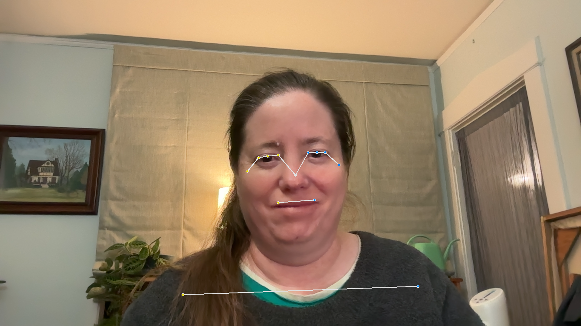
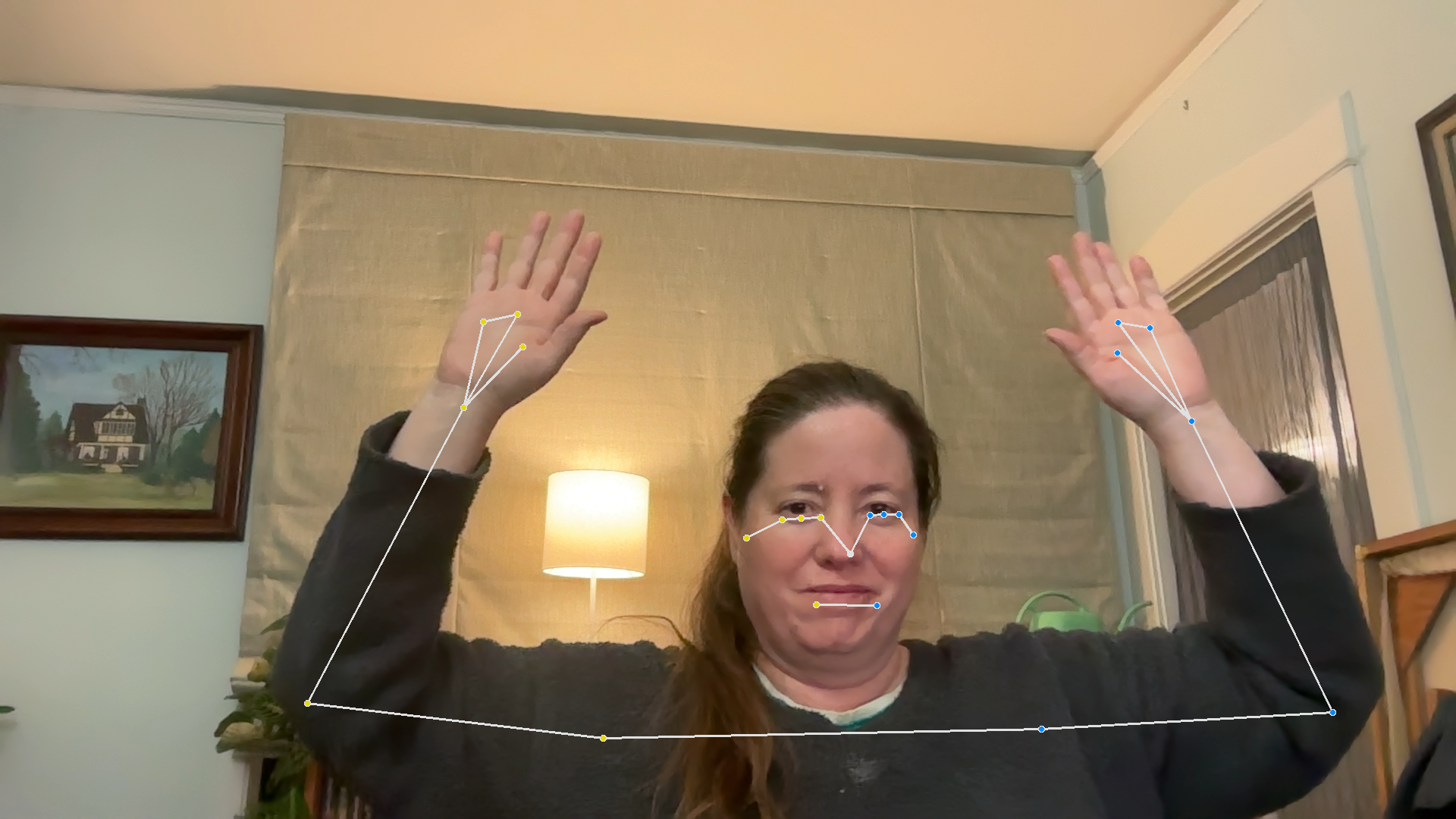
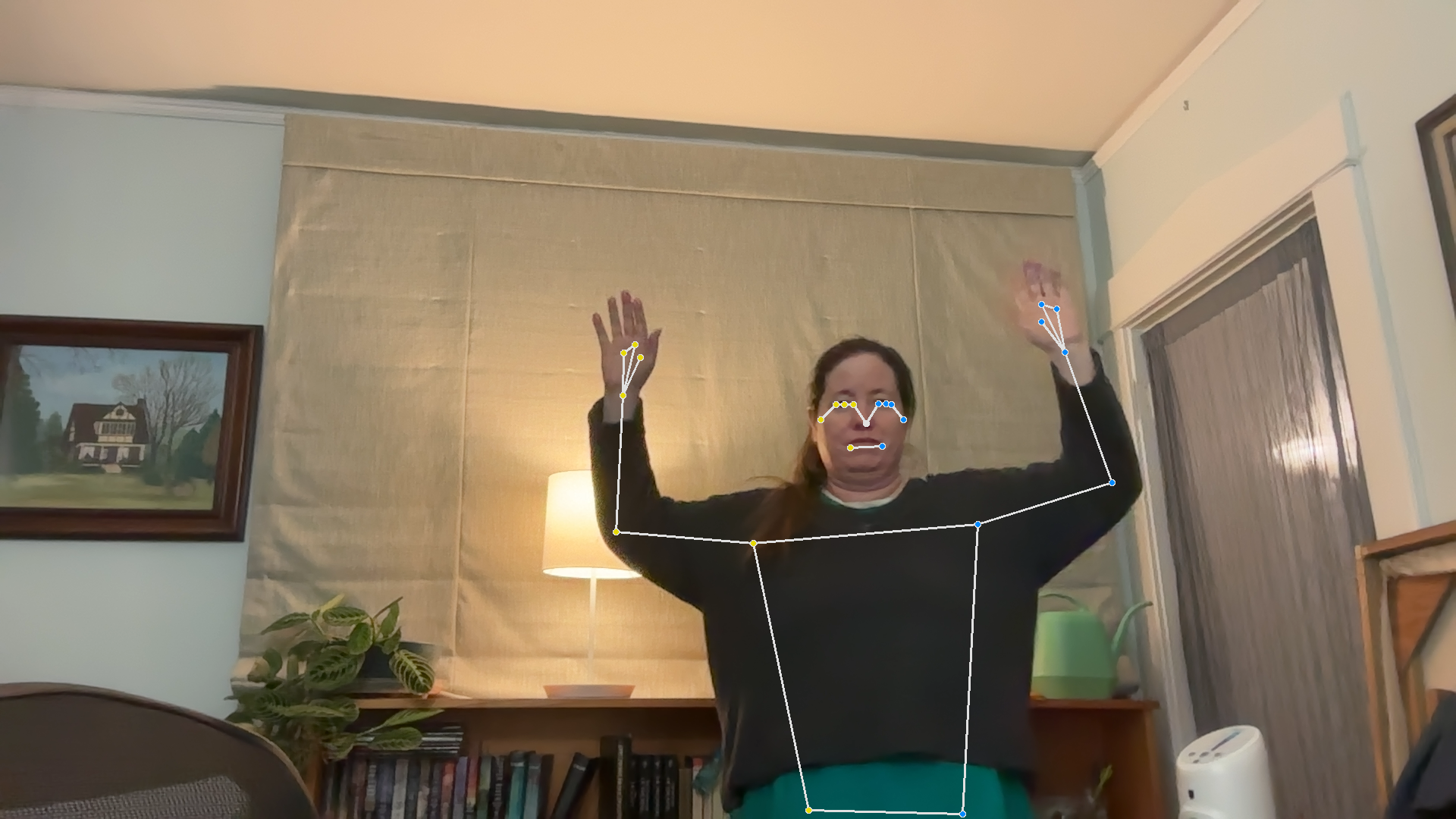
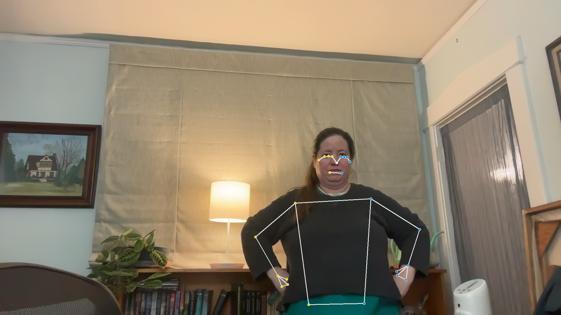
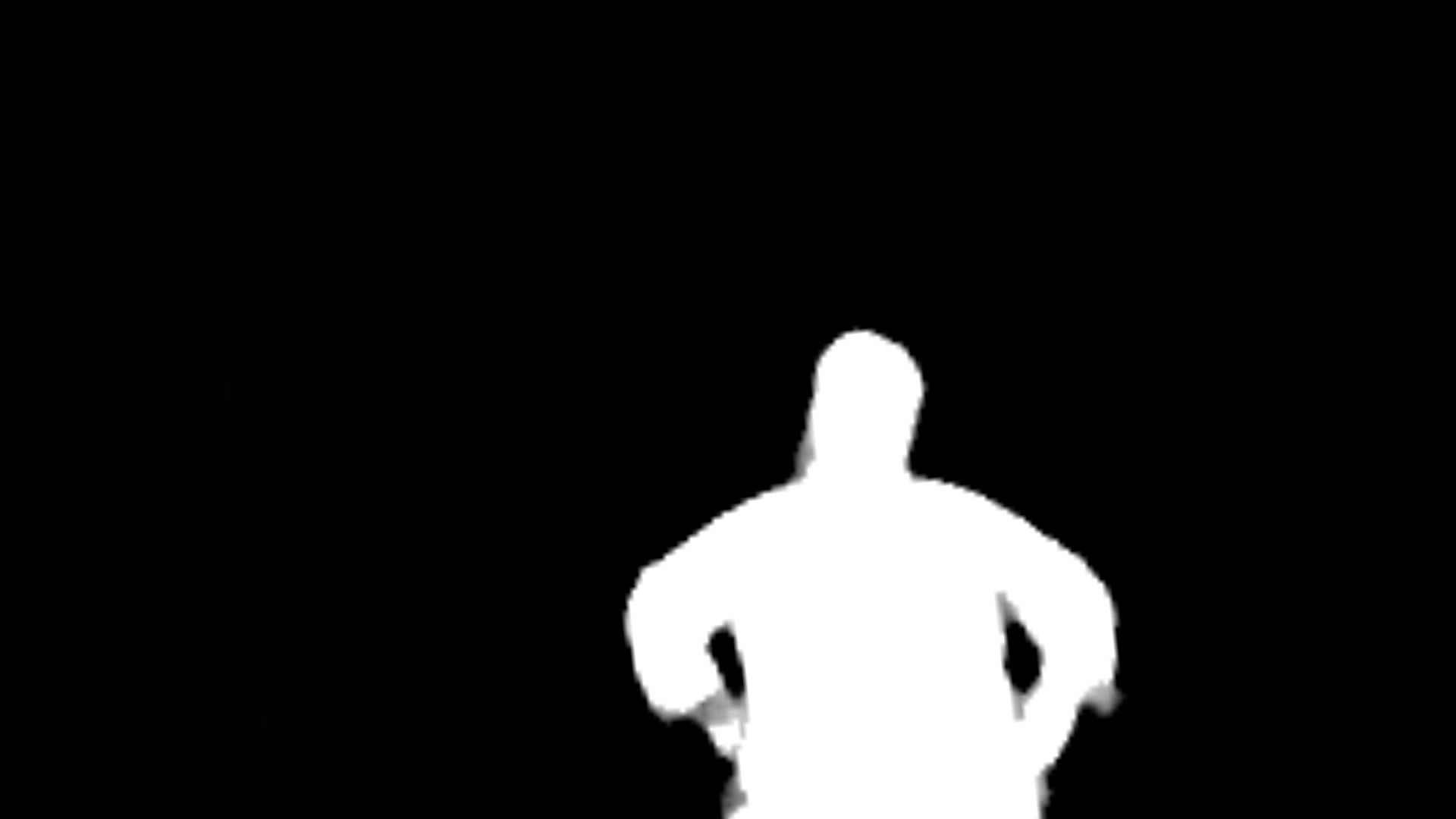
Figure 7 shows several screenshots from the running of this program, showing both the skeleton drawn onto the original frame, and also the segmentation mask, which shows the region of the image where the model thinks a person is. Note that the model’s default options look for one person, and not every person in view.

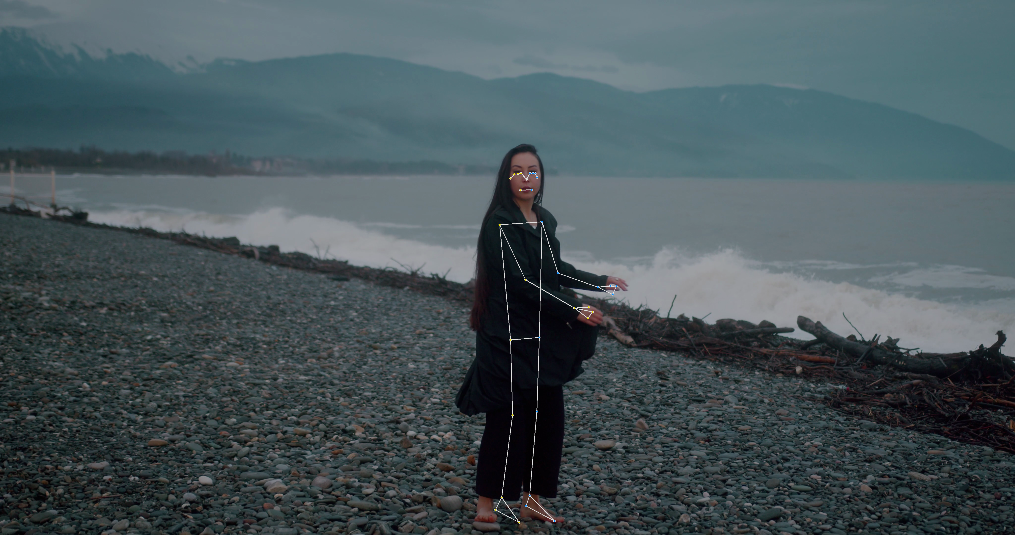
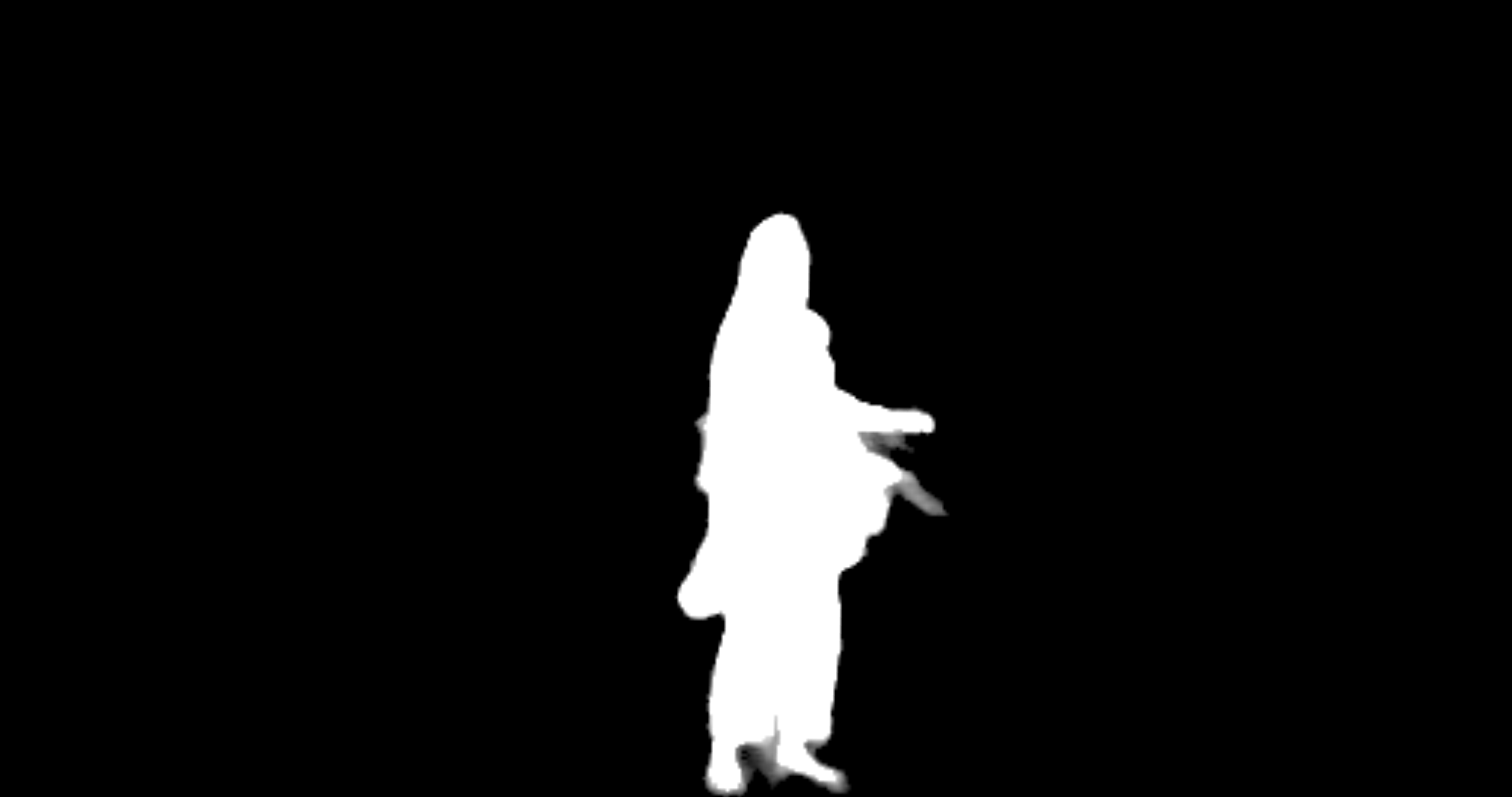
Figure 8 shows the skeleton and segmentation for a more distant view of a person

1.4.1 Examining the body pose landmark detection program

This program has three functions, plus a short main script that calls the main function.

The runPoseDetector function is the main function. Like the other demo programs, it sets up the pose landmark model and then uses it on frames from a video feed. It includes a commented-out function that can interpret the results from the model, if you choose to work on this program.

The visualizeResults function draws the results on the current frame. It uses Mediapipe’s more sophisticated drawing tools, in order to draw the skeleton and the 3d points most easily.

The findHandsUp function is for you to implement, if you choose. It would try to distinguish between hands above the head versus below.

1.4.2 Body pose landmark results

The results returned from the body pose landmark detector are similar to the hand landmark detector. The landmarks are given in two forms, as normalized landmarks and as world landmarks, a third part of the result (optional) holds a segmentation image mask, showing where the person is.

Accessing results	Explanation
`dt = detector.detect(mp_image)`	`dt` is a `PoseLandmarkerResult` object. It has three variables within it: `pose_landmarks`, `pose_world_landmarks`, and `segmentation_masks`.
`pLmarks = dt.pose_landmarks`	`pLmarks` is a list of lists. Each sublist corresponds to one person detected, though the model by default detects only one person.
`pLmarks[0]`	`pLmarks[0]` is a list of `NormalizedLandmark` objects. It contains the 33 body pose landmarks, all given as 3d normalized coordinates. `NormalizedLandmark` objects, as seen before, have `x`, `y`, and `z` variables.
`wLmarks = dt.world_pose_landmarks`	`wLmarks` is the same as `pLmarks`, except that the data are represented as `Landmark` objects and the `x`, `y`, and `z` values estimate real-world distances (in metric)
`segImgs = dt.segmentation_masks`	`segImgs` is a list containing Mediapipe images. Each image segments one detected person from the rest of the image. The image contains floating-point values between 0.0 and 1.0. The higher the value, the more likely it is part of the person.

In the ICA code, there is a text file, poseLandmarkResults.txt that shows one example of the form of results.

1.5 Object Detection with Mediapipe (OPTIONAL CHALLENGE SECTION)

If you feel inspired, try out Mediapipe’s Object Detection model. Here are abbreviated instructions:

Read through and run the mediapipeObjects.py demo program
Print the results of running the model, and see what the structure is

2 Overview of Machine Learning

Machine learning can seem like magic when you first encounter it, and then it can be disillusioning to realize what “learning” by a computer actually is. While machine learning can be, on the surface, a simple idea, there are many variations, including the kind of task to be learned, the approach, and the outcomes. Whether or not machine learning corresponds to how people or animals learn, it has been tremendously successful in recent years, infiltrating many of the digital systems we work with every day, and having a huge impact on our society.

How to manage that impact, and AI systems, for the common good is a major study of AI ethics, which we won’t discuss here (it’s very important, and we’ll talk about it elsewhere!).

2.1 What is Machine Learning?

Machine learning systems comprise hundreds of different algorithms and approaches, but they are all fundamentally working on the same task: finding patterns in data. This is what machine learning boils down to. Most ML algorithms take in data, and look for statistical relationships among the data, and often between the data and the output to be learned.

A dataset is a collection of examples of the problem we want the ML system to learn. Most often, the dataset includes both input data and the correct answer, but sometimes it has only input data, or other more complicated configurations.

The main goal of a machine learning algorithm is to build a model that captures those statistical regularities. We want the model not only to give the correct outputs for the data in the dataset, we also need it to generalize to give correct outputs for new examples it has never seen before. That is the hard part!

2.2 Why use ML?

Some AI researchers explore machine learning because they want to understand learning better. Perhaps that means simulating human or animal learning with the computer, or just exploring the limits of what machine learning can do, to illuminate our understanding of learning in general.

Most researchers and practitioners in industry, however, turn to machine learning to solve a problem because we don’t know how to solve the problem otherwise. A problem that is large and complex, or poory-specified, often cannot be solved by building an algorithm by hand. Computers are much better at finding statistical patterns in large, complex data than we humans are.

2.3 Kinds of machine learning for computer vision

Other resources will discuss the differences between supervised, unsupervised, and reinforcement learning, as well as hybrid variations like self-supervised, auto-associative, and semi-supervised learning. Here we will focus on what those variations look like in the context of computer vision tasks.

2.3.1 Supervised learning in computer vision

Supervised learning is the most common kind of machine learning. The ML algorithm is given both input data, often an example of a problem to be solved, and also the correct output. The task is just to learn how to map the input example to its corresponding output.

In computer vision, supervised learning is also the most common results. Common tasks include image classification, object detection, and image segmentation.

For image classification, the input is an image, and the output is a category that the content of the image falls into. Categories could be things like digits, for hand-written digit recognition, or ASL letters, or animals we want to identify (cats versus dogs, bird species, butterfly or moth identification). This is the most common and versatile approach, and the most straightforward. Inputs are typically a single image, and the output is a code that indicates the category or class the image falls into. Imagenet is an example of a very large image classification dataset: it contains millions of pictures, each classified as one of 1000 categories.

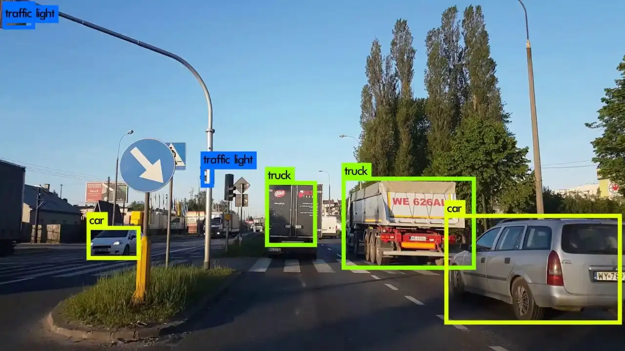
Object detection is also addressed with supervised learning, but the output is significantly different from classification. With object detection the output is a list of bounding boxes, rectangular regions that contain an identified object. Each bounding box has a category associated with it. Figure 9 shows a sample output from an object detection model that has been trained to identify vehicles from a dashcam video (a common task for autonomous driving systems). This example shows the category assigned to each object. Often we have a confidence value for each object, as well, indicating how sure the model is that it has correctly identified an object.

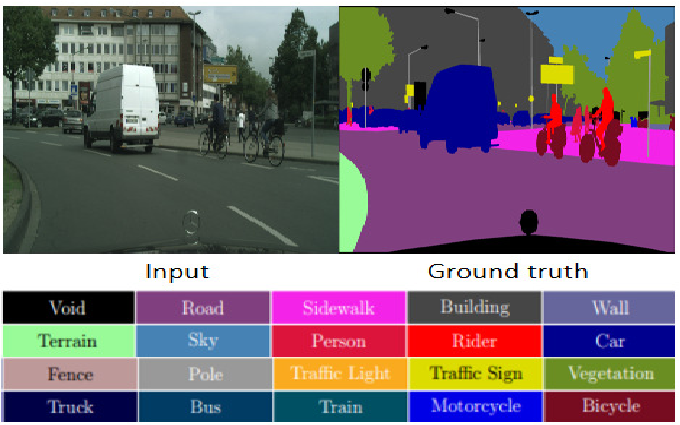
Object detection provides a more detailed output than classification: while classification associated the whole image with one label, object detection detects multiple objects, and identifies their class and location in the image. Image segmentation takes this one step further, and labels each pixel with what object it belongs to. Figure 10 shows an example segmentation. Segmentation gives us the most detailed response, but is the most difficult task for the machine learning system.

2.3.2 Generative AI for images

Generative AI systems contain, at their core, a large model trained on an incredibly large dataset. They are typically trained with a self-supervised approach where the target output derives naturally from the dataset itself. So for natural language text, the model is typically given a sequence of words, and asked to predict the next word (or sometimes to fill in a blank in the sequence). For image generators, the nature of the target depends on the method used. One top method, diffusion, relies on adding random noise to an image, and then asking the model to recreate the original image from the noisy one. This is an example of auto-association, because the target is the same as the original input.

Generative AI systems include some that work with multiple modalities (text, images, audio, video, etc.), while others focus on just one modality, such as images. While Generative AI systems are more complex than models that perform image classification, or even object detection or segmentation, they often use the same convolutional building blocks to perform their tasks. We’ll take a look at how these models work in a later section.

3 Convolutional Neural Networks

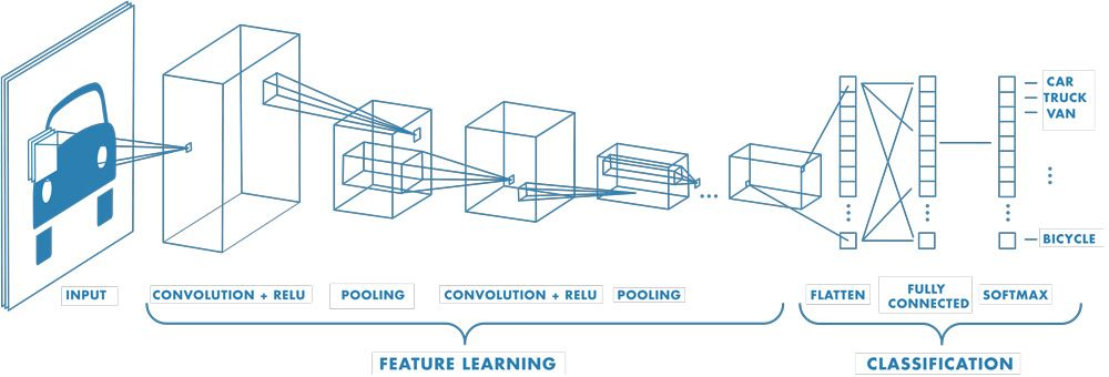
Convolutional neural networks introduced a number of operations that have become the foundation for almost all deep learning computer vision models. The most simple models, which we’ll examine here, perform image classification. Figure 11 shows the parts of a typical CNN model.

To run this model, we input an image (shown on the left). The image data passes through multiple layers that seek to extract meaningful features from the image (much like the work we did with blurring, morphing, edge detection, etc.). At each point the data is transformed either by convolutional filters or pooling, where the data is reduced in size. Finally, the condensed representation of the image and its features is passed through several final layers that use the features that were detected to determine the class the image belongs to. The final output, on the right of the model, is a real value for each category. The value represents the likelihood that the input image belongs to that category. If we look at the largest output value, it corresponds to the most likely class for the input image. We can also interpret the output real number as the model’s confidence in its classification: the higher the value, the more sure the model is that it is classifying correctly.

Running the model is a complicated and computationally-expensive task. Training the model is even more so. We will take up the question of training a CNN in a later section, after discussing the layers that make up the model.

3.1 Convolutional network layers

A typical CNN is built from a set of 4-6 typical layers, although dozens of variations and additional layers have been invented. The main layers include (1) convolutional layers, (2) pooling layers, (3) a flattening layer, and (4) dense layers, plus optional dropout layers, and the special dense layer that comprises the output layer, usually defined to perform the softmax operation.

3.1.1 The convolutional layer

A convolutional layer contains a set of independent convolutional filters, all using the same neighborhood size. Each of these filters has its own kernel, and applies that kernel to the input data, producing a single-channel feature map whose values are based on the weighted sum of the kernel with each overlapping neighborhood in the original image. The filter is applied to a small region of the image, and performs a weighted sum of the weights with the values in the region. We then slide the filter all over the image, computing the weighted sum at each location, and we produce a feature map where larger values indicate the presence of the feature the kernel is looking for.

If we have 20 filters in a single convolutional layer, then the output of the layer will be 20 channels deep: one channel for each feature map created by the 20 separate filters. The results of the convolutional filters are modified additionally by the Relu activation function. Relu, which stands for Rectified Linear Unit, is nonlinear, which is mathematically important for the model to learn any pattern. When given a value from one of the filters, it converts all negative values to zero, and leaves all positive values alone.

Each filter has a kernel, a matrix containing weights. These weights identify interesting features in the image. Convolutional filters can be used to identify edges, as we have seen, but also to detect color patterns, stripes or lines with specific orientations, or circular/semi-circular patterns. These simple patterns may then be combined by later convolutional layers to detect complex patterns.

When training a model, the kernel weights are set initially to random values, and then the weights get tweaked by the training algorithm to make the model work better.

3.1.2 Pooling layers

Pooling layers reduce the size of the data that comes into them, without modifying the number of channels. This is sometimes called downsampling in computer vision terms. The pooling layer divides the image into small patches of a fixed size, not overlapping with each other. It then keeps one value from each patch, reducing the size of the image correspondingly.

The most common kind of pooling is max-pooling: given a small region of an image, it keeps only the largest value. Suppose that our pooling patch size is 2 by 2. We keep one value from this patch of four values, reducing the height and width of the image to half their previous size.

Why do we need pooling?

The main reason to perform pooling has to do with the nature of convolutional filters. It turns out that these filters work best and most efficiently when we keep the neighborhood sizes very small (3 by 3, 5 by 5, possibly 7 by 7). But suppose there are patterns in an image that are larger than that neighborhood size! The small filters can’t see them. We can’t really increase the size of the neighborhoods to guarantee that we can detect every such pattern. But if we scale the image down, then the features will eventually become small enough to be detected by the filters. This is called building an image pyramid, and it has its uses from earlier, algorithmic approaches to computer vision, before the growth in deep learning.

3.1.3 Other layers to know about

Drop-out layers help with overfitting by blocking some data from passing through them. At any particular time, a drop-out layer choose a random number of values to block (a percentage given when we create the layer). This forces the model to incorporate redundancy into its operations, requiring it to generalize more.

Softmax layers are typically used for the output layer. They take the values computed by the weighted sum and run through the Relu activation function, and they scale them so that the values are all between 0.0 and 1.0, and they add up to 1.0. This lets us treat the values as probabilities: the likelihood that each output unit is the correct label for the current input. We can pick the largest probability as the model’s guess for the category, and we can treat the model’s value as reflecting its confidence in its answer.

3.2 CNN training process

When we create a new neural network, we set all the weights within it to random values. Then we want the model to make small changes to its weights in response to each example, based on the details of the **loss*, or error, between the model’s output and the target output we want it to make. It make a small change to each weight to make the model closer to producing the target value.

The change in weights has to be small, to balance the changes that need to be made across all the images in the dataset. If we made large changes, the model could end up swinging from weights that work for one particular image, to weights that only work for a different image, and back, without finding a compromise set of weights that work for both images.

We present all the images in the dataset to the model, and update it as we go with changes to its weights. We call that one epoch in the training of the model. Training a neural network requires us to run through the dataset multiple times, for multiple epochs, until the performance of the model is sufficient, or stops changing. For a small model and a small dataset, we may only need to run the model for 10-20 epochs. For larger, or more complex tasks, we may need to traing the model through hundreds or even thousands of epochs.

3.3 CNN Examples

While CNNs are simple enough that we can build small ones from scratch, there are many existing CNN architectures that have been applied to many problems and proven broadly effective. These include VGG and Resnet, which are both older models. Google’s Inception models are too large for practical use, but worked very well. More recently, architectures like MobileNet, DenseNet, and EfficientNet have become standard.

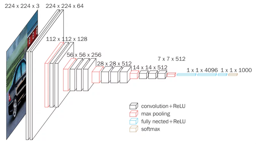
Figure 12 shows the structure of the VGG architecture. It uses only the kinds of layers we discussed above, and has limited numbers of each kind of layer. Nevertheless, it works well on many smaller tasks, and is often a good choice to try before attempting a more complex model

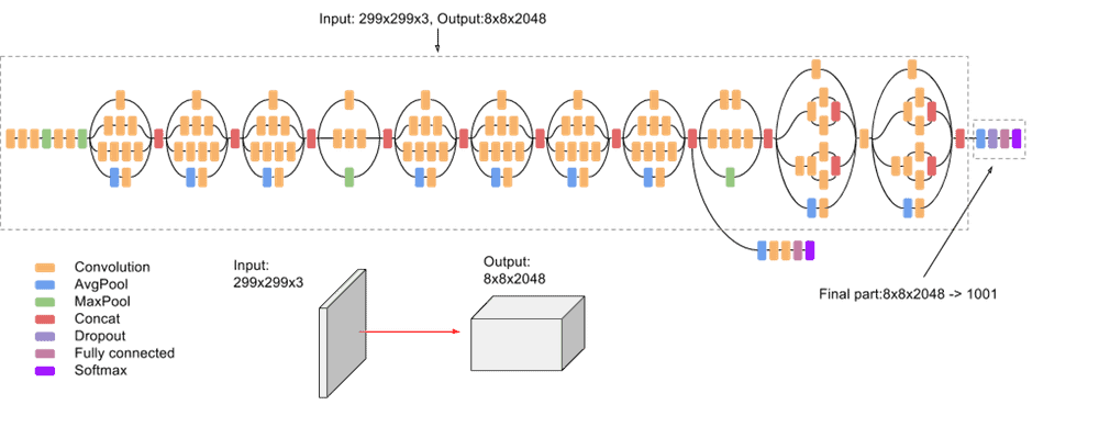
At the other end of the spectrum, Figure 13 shows Google’s Inception version 3 model. This model has a complex structure and many many layers. It was highly successful at learning and generalizing from the Imagenet dataset (with 1000 classes and millions of sample images). Because of its size and complexity, Inception v3 was difficult to run on an ordinary laptop or desktop machine, and it had to be trained with a supercomputer or the resources of a data center.

Since Inception v3’s creation, work shifted to models that were smaller, lighter-weight, and yet could work well. EfficientNet and Densenet are two general-purpose architectures, while MobileNet was explicitly created to be small enough to run on a mobile device.

3.4 How will we work with CNNs?

Because even smaller CNNs are best trained on a system with access to powerful GPUs, we will be using Google Colab to train CNNs for some straightforward image classification tasks. Colab is available for free: with it, we can create Python programs that run on a machine from one of Google’s data centers. All the machine learning libraries we need are provided in Colab, and we have access to Google’s GPUs to speed up the training process.

Colab uses a notebook model for Python programming. The notebook integrates text blocks and code blocks, and allows us to run each code block individually. While the can be run separately, all code blocks operate in the same global space. Variables defined in one block are available in all the other blocks that run afterward. This leads to a more script-heavy programming style than we have been using thus far. But this is what a large percentage of data science work in Python looks like these days.

3.5 Where do the datasets come from?

It is fairly easy to create a dataset for image classification: collect a huge number of images, and then sort them by category into separate folders, one folder for each category. Many CNN libraries come with functions that can read data in this structure automatically, but it also isn’t too difficult to write a few functions that would read in images stored in this way, and associate each with a number assigned to the folder they came from (you could do it!).

The biggest issue is the large number of images we need for successful classifications, and the need for accurate categorizations. For large-scale problems, the work of assigning each image to a category is outsourced, either to volunteers or, through websites like Taskrabbit or Amazon’s Mechanical Turk, to people being paid a small amount for each image processed. Maintaining accuracy under these circumstances is a huge problem. There are also ethical issues with the low pay rate workers receive for this work.

4 Object Detection and Segmentation Models

Object detection and image segmentation are two tasks that machine learning models have been able to tackle successfully, while traditional algorithms have not worked well.

We have seen examples of color tracking, like Camshift, that detect the location of a colorful object in an image or video. You’ve experimented with detecting coins and balls in images using various computer vision techniques (thresholding, edge detection, finding contours, etc.). You’ve also experimented with motion detection and background subtraction as ways of identifying where important foreground objects are in an image. You’ve also seen how glitchy, finicky, and incomplete these methods can be.

Deep learning neural networks perform so much better than the alternatives.

4.1 Object detection in the context of deep learning

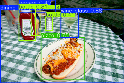
Object detection systems take in an image or frames from a video, and they identify any number of objects in the image (usually there is an upper bound in practice). For each object, they categorize it into one of N classes, the categories it knows about, and they draw a bounding box, a rectangle that contains the object. Figure 14 shows an example of the output of an object detection model trained on the COCO dataset.

Notice that the bounding boxes overlap, and are very different sizes. Also notice that the results are not completely accurate, and the model outputs a confidence value as well as the bounding box and category. It is only 75% confident that the foreground object is pizza, and mis-identifies something as a person, but with only 40% confidence.

Object detection neural networks have several different structures, but all of them incorporate feature-detection sections like the CNNs in the prevous section, as well as dense, fully-connected layers used to classify features. Here, those classifications happen repeatedly for each bounding box that was discovered.

We will focus on one example of an object detection network: the YOLO (You Only Look Once) family of networks, developed by the Ultralytics company, and freely available through them. Ultralytics has developed a whole series of YOLO models (up to version 11 currently) for both object detection and image segmentation tasks.

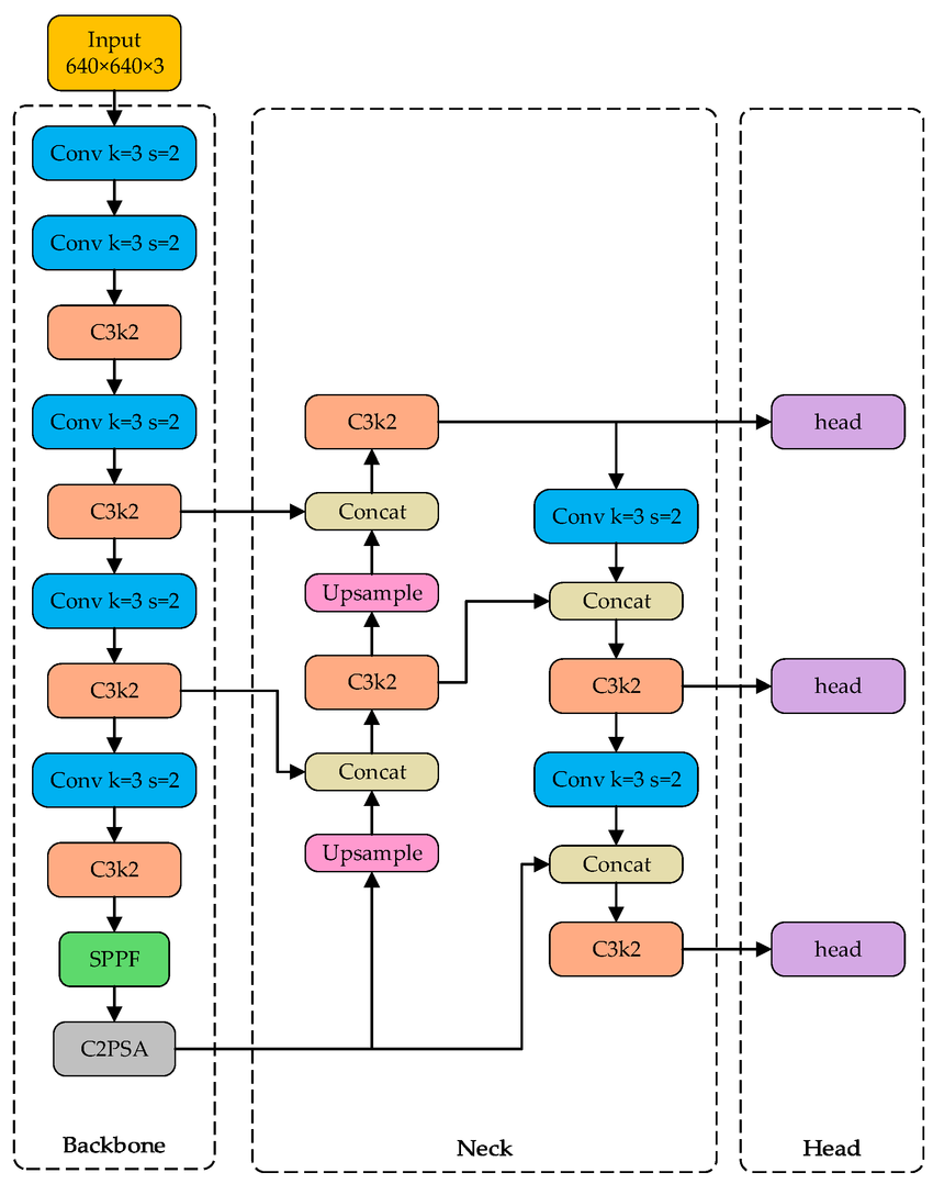
Figure 15 shows a diagram of the YOLO version 11 model (you do not need to grasp all the details here).

The Backbone section on the left is similar to a CNN feature detection component, although it has some special-purpose layers (C3k2, SPPF, C2PSA) that, themselves, involve convolutional layers and smaller special-purpose layers. The purpose of the backbone is to identify interesting features in the image at different scales, places where objects to be identified might be. Information from different scales is passed from this part of the model to the Neck section. The Neck integrates the information from different scales. Concat layers just combine multiple values together, Upsample scales an array up to a larger size, and so on.

Finally, information at different scales is passed to the Head units, which perform the classification (or segmentation) on the regions identified to be of interest. The Head produces the final output.

One reason that YOLO is so popular is that Ultralytics has made it extremely easy to load pretrained models (models that they have trained on general-purpose datasets), and also to retrain them (usually called finetuning) on new data. YOLO models are larger than ordinary CNNs, though, so we really need cloud resources to work with them.

4.2 Image segmentation

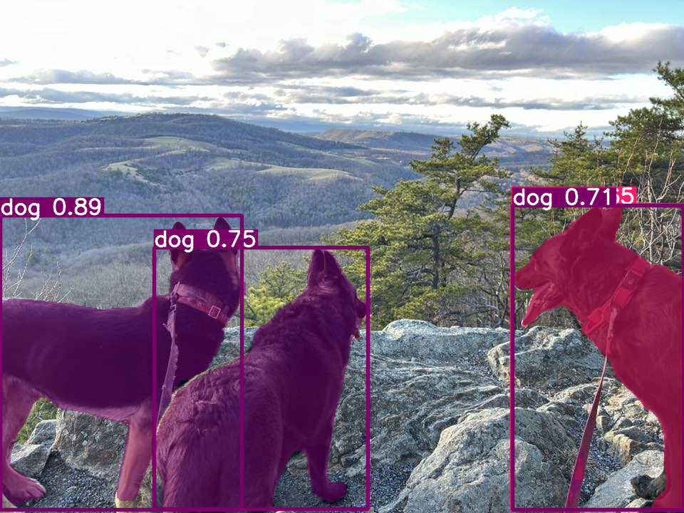
Image segmentation is a harder task than object detection. An image segmenter outputs a copy of the original image, where each pixel belonging to an object that has been detected is marked with a code that indicates its object. A segmentation of an image is like a mask, except that instead of being black and white it is typically black for background pixels, and then a set of colors, one for each detected object. Figure 16 shows the result of using YOLO’s own display function to show the result of the segmentation. It shows both the object detection values, and tints each pixel in the original image to show the segmentation.

The dog on the right is shown in a different color because the system is confused. It thinks it could be a dog, but behind that on the picture is drawn another classification: it thinks the dog on the right might possibly be a horse. That is why it is shown in a different color.

4.3 Where do the datasets come from?

The YOLO models about were trained on the COCO dataset, one of the classic datasets for object detection and segmentation. This dataset, called Common Objects in Context, has over 300,000 images, each of which may have multiple objects in it, for a total of 1.5 million annotated objects. Each object is assigned to one of 80 object categories. Each image also has five captions that describe the scene. More than 200,000 of the images are annotated: the bounding boxes, categories, and segmentation maps have been created by hand. This is a large dataset, took a tremendous amount of work to create, and requires massic computational resources to use.

We noted in the previous section that image classification datasets are relatively straightforward to create. That is not the case for object detection and image segmentation datasets. These models are still supervised learning systems. They must be given the correct answer in order to train them to perform the task. That means that someone has to annotate each image in the dataset with the bounding boxes, or paint the pixels for the segmentation. This is painstaking work, particularly given the large size needed for these datasets.

There are online tools available to help with this annotation. Some of them even integrate AI models that already perform object detection or segmentation for some general task, and then try to learn from your initial annotations what it is you want. These help, but still the task of building a dataset for object detection is extremely difficult.

5 Image-generating models

Generating images might seem quite different from processing images to recognize objects in them, but it turns out that similar underlying methods actually come into play. Generative AI models use convolutional and pooling layers, at least during training, along with upsampling and other specialty layers as well.

5.1 Encoder-decoder models

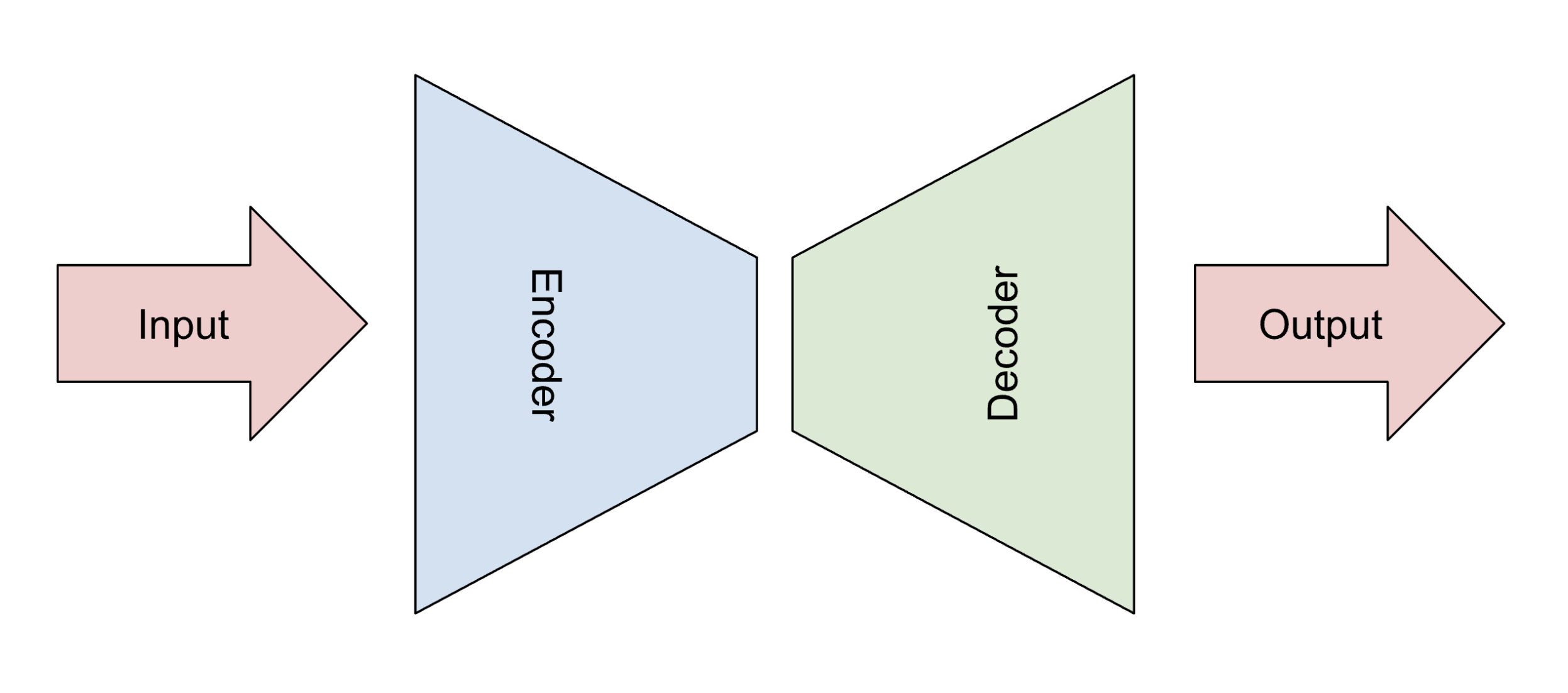
Image generators grew out of work on encoder-decoder models. These models look, generally, as shown in Figure 17.

The first half of the model might be like the CNN feature-detector part, or the backbone of the YOLO model. It converts the input image, or any kind of input data, into an encoded form, usually significantly smaller than the original image.

Then, the decoder part of the model unpacks the encoded form into the final result. The final result might be any number of different things: perhaps a text description of the input image, or a segmentation map of the original image. One of the most curious target outputs is to have the model output the same image as was input. This is called auto-association.

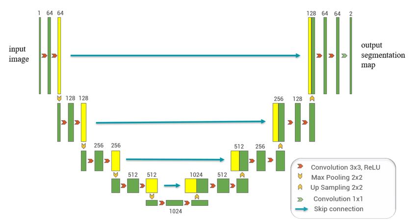
A common encoder-decoder model for computer vision is called the U-Net. Figure 18 illustrates this architecture. The left half is the encoder, and it is essentially the same as a CNN feature detection component. The second half is the decoder, and it reverses the pooling effect by upsampling the data, while incorporating some of the data generated by the encoder at corresponding steps.

Why would we want to build a model that takes in an image and output the same image? Precisely because of the bottleneck at the center of the encoder-decoder shape. If we can decode the pattern into the original image, then that pattern represents all the important information from the image, in a condensed form.

Once the model is trained, we can split the model into two pieces. A common use is data compression: we can use the encoder to build a compressed representation of the image, transmit that to a new location, and then use just the decoder to reconstruct the original image.

Another less obvious use for the decoder is image generation. If we build a random array or vector in the style of the encoder’s output, then the decoder may unpack it into a brand-new image!

This allows us to produce new iamges, but usually not very good ones. Two more complex architectures have followed on the basic encoder-decoder model, with remarkable success: Generative Adversarial Networks (GANs), and Diffusion models.

5.2 Generative Adversarial Networks (GANs)

GANs were the first highly successful image generators. They could make recognizable images, though they were more liable to have strange artifacts (too many fingers, strange shapes intruding) than later models.

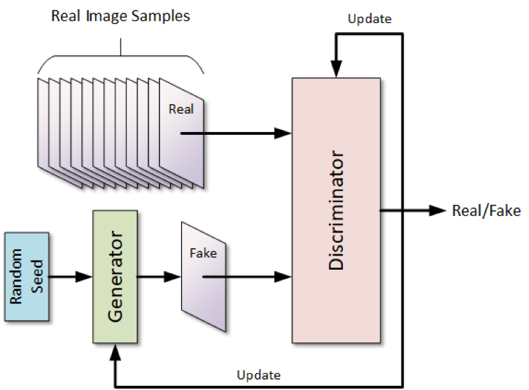
With a GAN, we actually are training two separate models in tandem with each other: the Generator, and the Discriminator. Figure 19 shows a typical GAN architecture.

We have a dataset of real images, and we want to train the models to generate and assess images of that type. The generator model takes in random noise, and it generates an image based on that noise. The discriminator is given an image, which is randomly chosen to be either a real image or a fake one created by the generator. The discriminator’s task is to correctly identify real from fake images. If the discriminator correctly identifies the output from the generator as fake, then it has low loss, and so isn’t change much, but the generator is given a large loss, pushing it to do better. If the discriminator outputs the incorrect answer, then it has a large loss, and the generator has a small loss.

The two architectures develop in an adversarial way, each one pushing the other to improve.

Once the model is trained, we can extract just the generator, and use it to generate new images.

GANS were notoriously difficult to train: they were finicky and the two models could collapse into a situation where one or the other always won. They also couldn’t get rid of certain artifacts that immediately identified the output as computer-generated.

5.3 Diffusion models

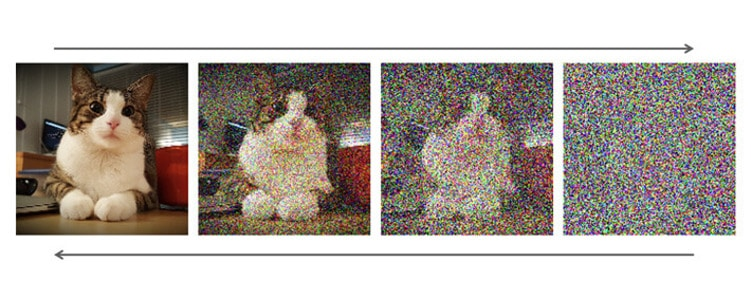
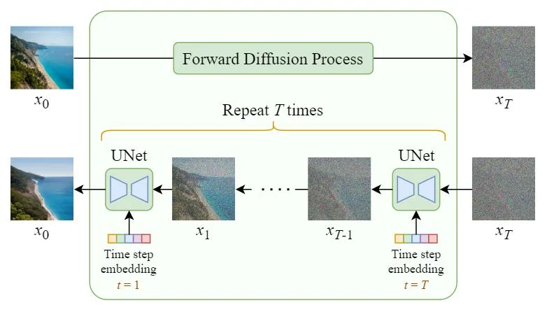
Diffusion models are at the heart of current state-of-the-art image generators. The general idea is fairly easy to understand, though the details are more complex. Figure 20 illustrates the general process.

The input to the model is an image, and in the encoder phase it passes through a sequence of steps that add random noise to it. Each increasingly noisy image is saved. (No learning happens in the encoder phase.)

In the decoder phase, the model learns to transform each noisy image into its predecessor image in the sequence. Let’s take a closer look at the diffusion architecture to see how that works. Figure 21 shows the pure diffusion process. Once the model is trained, we can use just the decoder half to generate new images: we provide random noise in the shape of an image, and generate a new image from that.

In between each pair of noisy images the pure diffusion model has an encoder-decoder model, in this case, a U-net. The sequence of U-nets is trained to reproduce the original sequence of noisy images, but in reverse order. The U-net model does also take in additional data, in this case an input that tells it what staget in the process it belongs to.

Pure diffusion worked better than GAN models at generating realistic-looking images, and it was somewhat easier to train. But training a whole sequence of U-nets was very expensive!

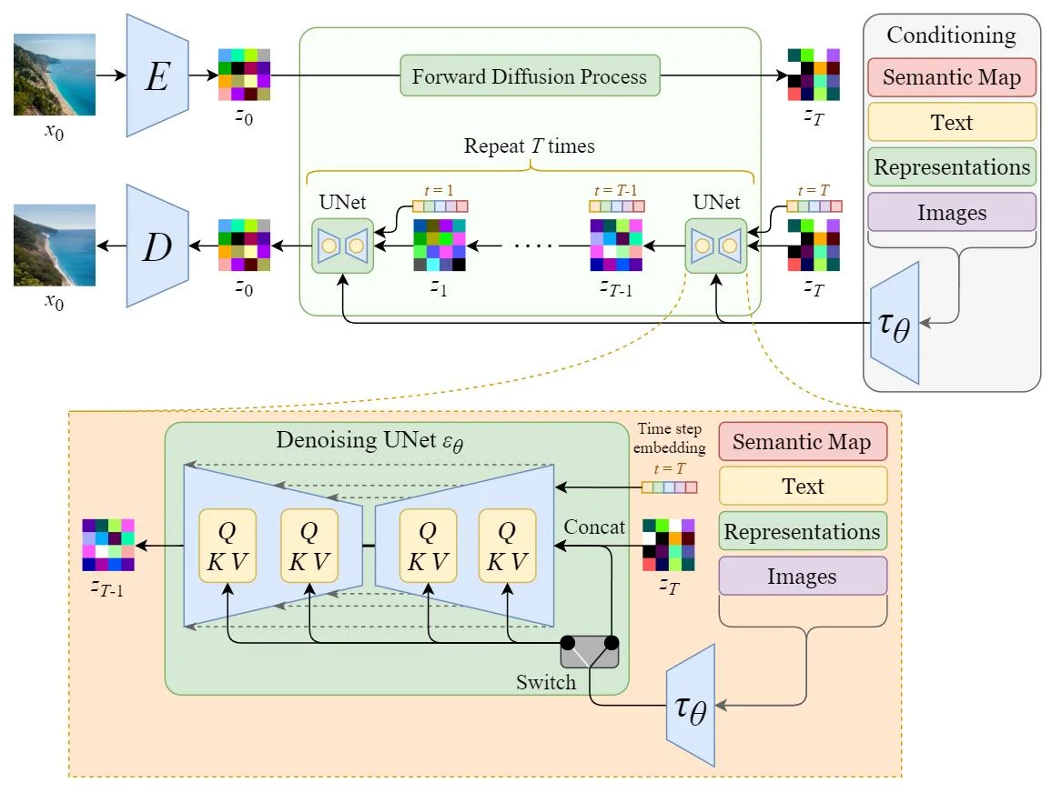
Stable diffusion introduces another layer of complexity, but it works much much better than its predecessor, and is much more efficient to train. Stable diffusion assumes that we already had an encode-decoder model trained to perform autoassociation. We use the encoder part at the start, to convert from the original image representation to the condensed, compressed representation. We call this a representation in latent space. We then add noise to the latent representation, and train the decoder half of the diffusion process to produce from one noisy representation the next less noisy representation. At the very end the decoder half of the autoassociator converts from the latent representation back to an image representation.

Notice that, once again, the networks between each pair of noisy representations is a U-net. Each U-Net combines the latent representation with other data, such as the text guiding what should be produced, which is encoded separately.

Once the diffusion model is trained, we can provide a text input, and some random noise, to the decoder half of the diffusion model, and it will generate a series of encodings, decoding the last one into an actual image.

Stable diffusion was a big step forward in image generation. Most current image generators use something like stable diffusion to perform their task.