Chapter 7, Detecting and Tracking Objects (without ML)
Author
Susan Eileen Fox
Published
October 29, 2025
This chapter will look at several approaches that allow us to identify objects in images, and to track motion and color. The first section will look at tools for finding and manipulating contours, arrays of (x, y) coordinage points that form a closed polygon on the image. The next section will examine basic motion detection, and background subtraction algorithms, and the third section will look at the Camshift color tracking algorithm.
(Later sections, if added, will examine line and circle detection, as well as corner detection)
1 Finding contours
All the image processing we’ve done in previous chapters has ended up transforming one image into another. The goal of computer vision is to get information out of images, but we haven’t really done that yet. Finding contours will be the first approach we will look at that does give us information. A contour describes a section of the image defined by a list of points. The points form a closed shape, a polygon. The polygon lies along a bright edge in the image.
The original contour algorithm was described in a paper by Satoshi Suzuki and Keiichi Abe in 1985 (Toplogical Structure Analysis of Digitized Binary Images by Border Following). The algorithm operates on a binary image, where all pixels are either white or black. If you give it a color image, its results are typically very noisy.
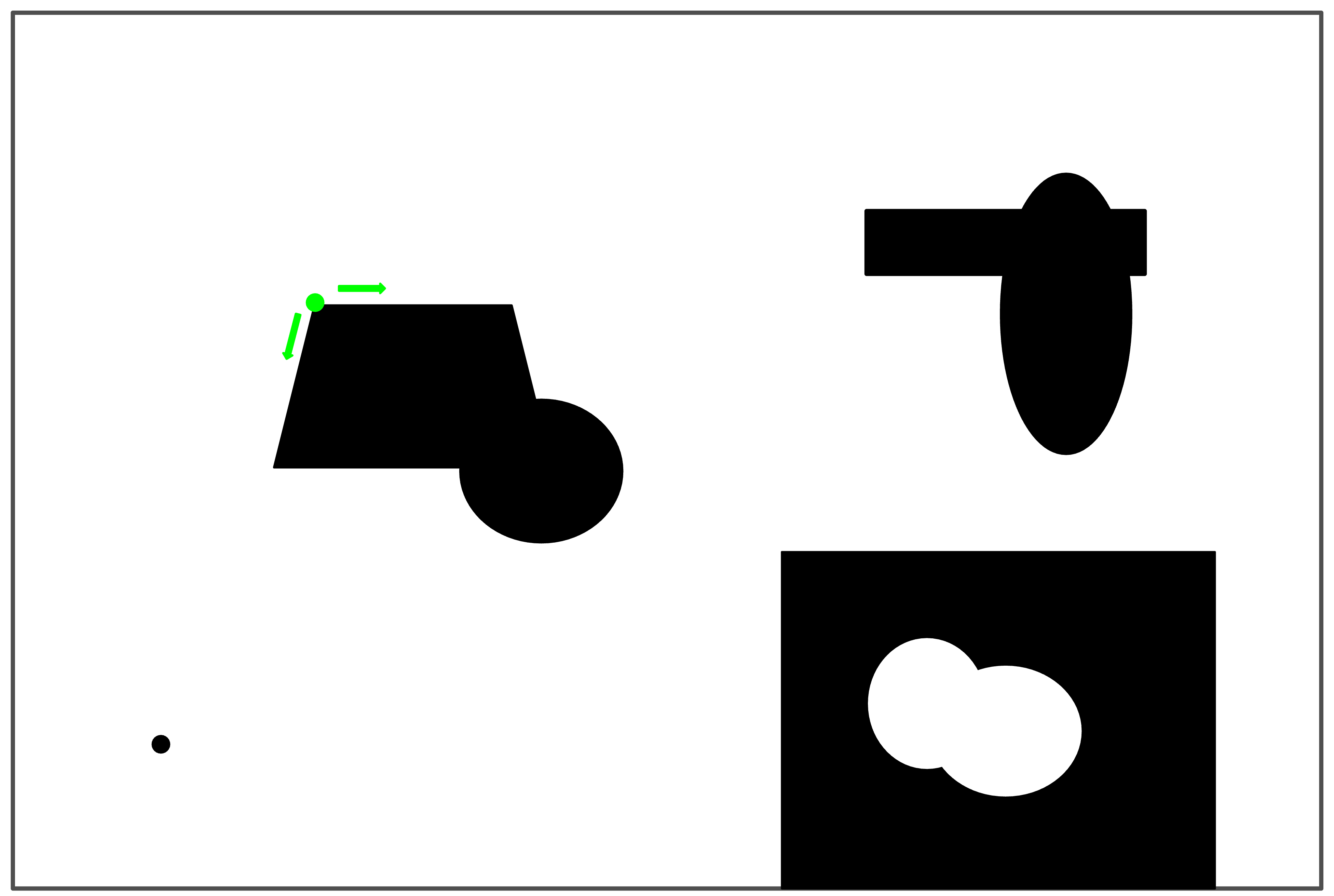
The findContours algorithm scans the image for a pixel that sits on an edge (where bright and dark meet) (as shown in Figure 1 below). It then determines neighbor pixels that are also edges, and follows the neighbors until it returns to the starting point, having traced a full closed shape on the image that lies along an edge. It repeats this task for the rest of the image, and returns a list of all the contours it found (as shown in Figure 1).
At the start, finding an edge pixel and searching for neighbors
At the end, having found five contours
Figure 1: Early and late in the contour-finding process
1.1 Inputs to findContours
OpenCV implements this algorithm with the findContours function. This function takes in three inputs, and returns two values. The three inputs are:
the binary image to be processed
a code specifying the mode of the search, and
a code specifying how much to approximate or optimize the contour that is found
There are five different modes for the findContours search, described in the table below. For our purposes, we will really only need cv2.RETR_LIST.
Mode
Meaning
cv2.RETR_EXTERNAL
Retrieves only outermost contours, doesn’t keep any contours inside of other contours
cv2.RETR_LIST
Retrieves all contours without any hierarchical information about which contours are inside which others
cv2.RETR_TREE
Retrieves all contours and constructs a tree representation of which contours are inside which others
cv2.RETR_CCOMP
Retrieves outer contours and connects them to holes in side of them but treats contours inside of holes as independent contours (CCOMP stands for “connected components” which is a mathematical term for these structures)
cv2.RETR_FLOODFILL
Uses a “flood fill” algorithm to build up regions of similar brightness or intensity, then makes contours of their borders (in essence, a completely different algorithm!)
The third input specified the “contour approximation mode”. This determines how much the contour is simplified. The two main modes are cv2.CHAIN_APPROX_NONE and cv2.CHAIN_APPROX_SIMPLE, though there are more complex modes that are rarely used. The NONE mode does no optimization or approximation of the contours. Every border pixel is included in the contour array. The SIMPLE mode looks for horizontal, vertical, or pure diagonal segments of the contour, and stores only the end points, rather than every pixel.
1.2 Outputs from findContours
As noted above, findContours returns two values. The first is a list of contour arrays, all the contours retrieved by the algorithm. The second return value is a hierarchy object that represents how contours are nested with each other. We won’t typically use this, but it does play a role in tasks like recognizing QR codes!
1.3 An example of findContours
The code block below contains a short example of how to prepare an image for findContours and what it returns. In the code, we read in a picture of a peony flower, convert it to grayscale, and then perform a simple threshold to split all pixels brighter than 80 to 255, and all darker to 0.
We then pass the threshold image to findContours, with typical mode inputs (cv2.RETR_LIST and cv2.CHAIN_APPROX_SIMPLE). We assign the two return values to the two variables contours and hierarchy. We won’t use hierarchy further.
The contours variable holds a list of contour arrays. Just to get a sense of them, the code prints the number of contours found, a surprising 68, and also print the values of the first two contours in the list. Each contour ach contour is an array of (x, y) coordinates, representing the pixels that form the contour.
Look closely at the contours that were printed. Each of them is only four pixels long. If you work out the locations of the four pixels, you will see that they form a diamond above, below, to the left, and to the right of a single pixel. These are the smallest possible contours, and usually not of interest to us. Many of the 68 contours are marking tiny patches of noise in the image (a demonstration of why we might want to blur or morph an image to get rid of these!).
1.4 Drawing contours
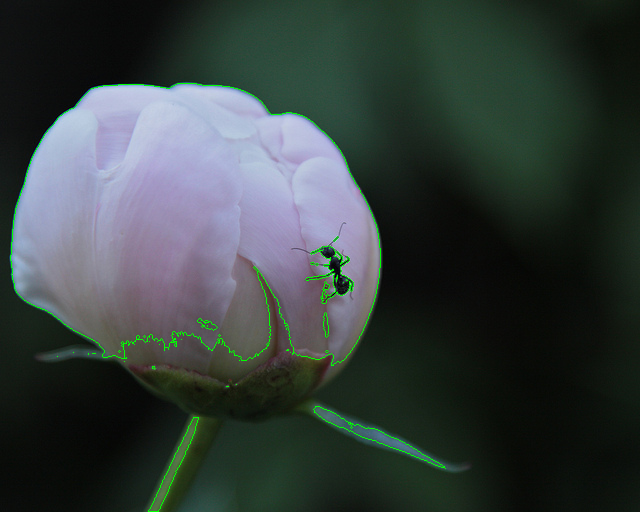
OpenCV also provides a helper function, drawContours for drawing contours on an image. The code snippet below makes a copy of the original flower picture, and calls drawContours on it to draw all the contours on it. Figure 2 shows the result of this code snippet.
an index into the list showing which contour to draw, or -1 if we want all contours drawn
A color for the contour polygon to be drawn with
A line thickness, or -1 for a filled in polygon
Figure 2: All contours drawn in green on the original peony picture
1.5 Selecting contours by area
We often need to reduce our list of contours to those that are of significant size to get rid of the noisy ones. The code block below, an extension of the previous one, introduces one of the many OpenCV functions that operate on contours: cv2.contourArea, which computes how many pixels are enclosed by a contour. We use it to keep only contours that enclose at least 100 pixels.
bigContours = []for contr in contours:if cv2.contourArea(contr) >100: bigContours.append(contr)print("Number of big contours:", len(bigContours))
Number of big contours: 4
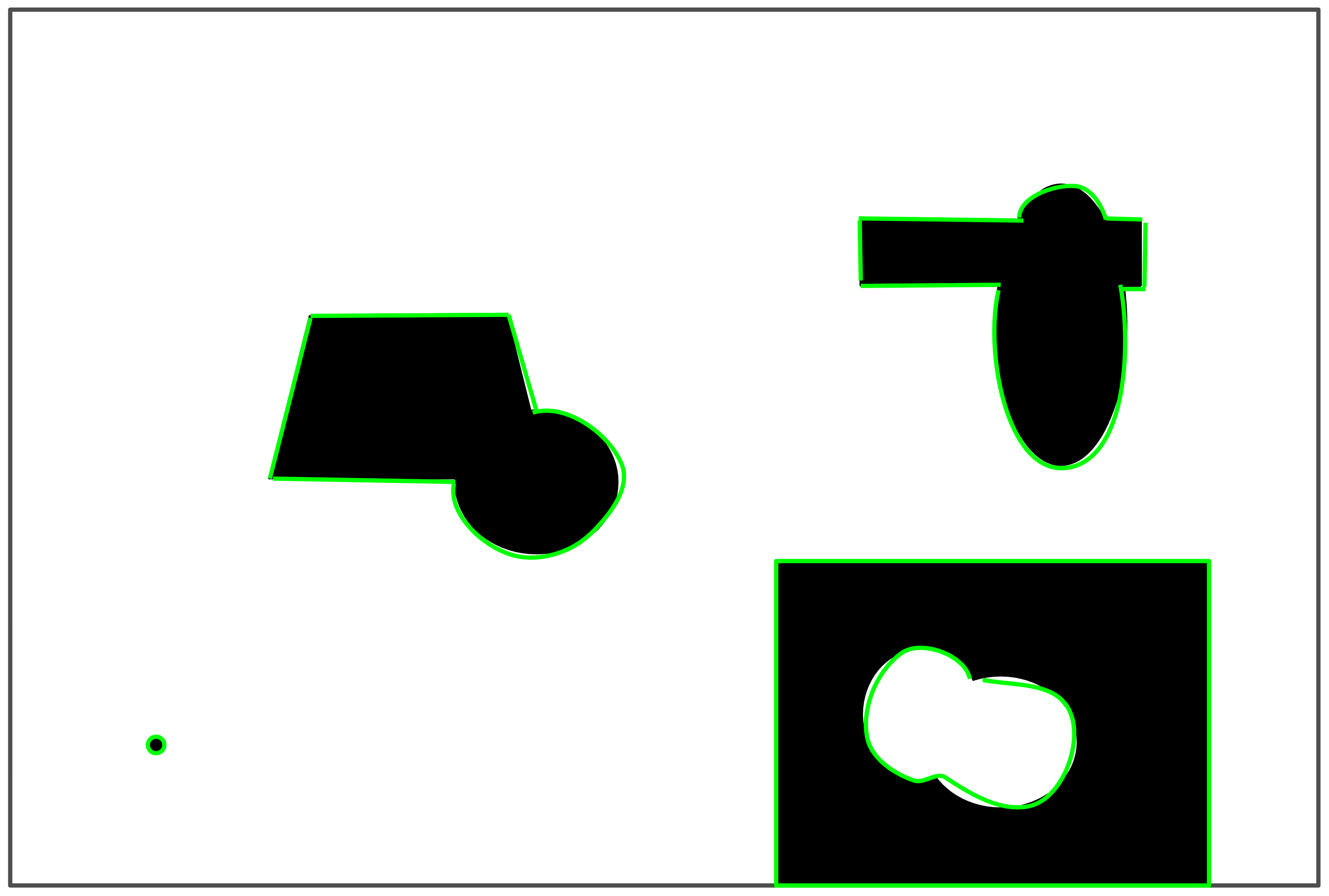
Figure 3 shows the result of drawing just the big contours on a copy of the original image.
Figure 3: Only contours with area above 100 drawn in green
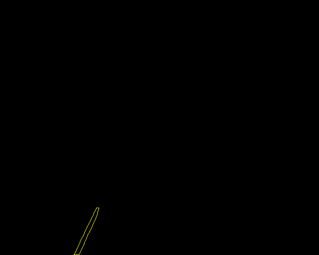
We can also view contours in isolation, by drawing them separately on either the original image or onto a blank image of the same shape. The code snippet below shows how to draw one contour at a time onto a black image. Note that the black image is recreated each time so that the contours show up separately from each other. Figure 4 shows each contour’s drawing, including one of the tiny contours that would included if this code ran on the full contour list.
for i inrange(len(bigContours)): bc = bigContours[i] blankIm = np.zeros(flowerPic.shape, flowerPic.dtype) cv2.drawContours(blankIm, bigContours, i, (0, 255, 255), 1) cv2.imshow("Contour", blankIm) cv2.waitKey()
Notice how the call to drawContours is different here. Instead of -1 for the index input, we are passing in an index into the list, so it draws only that contour onto the blank image.
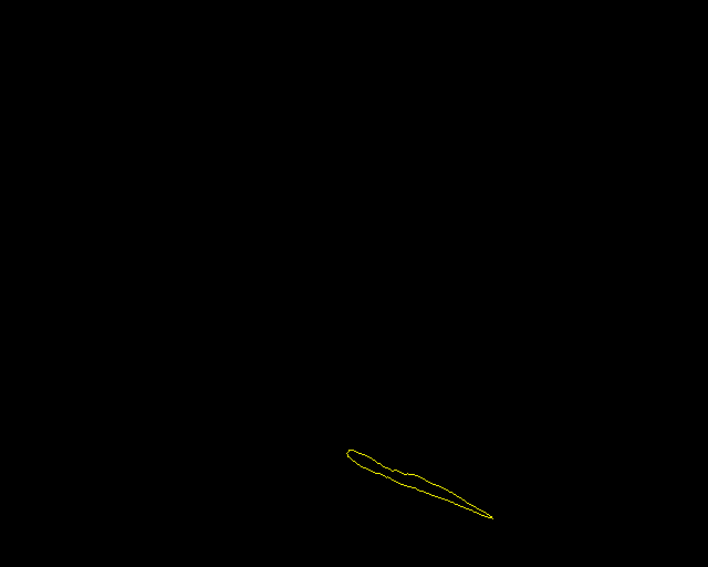
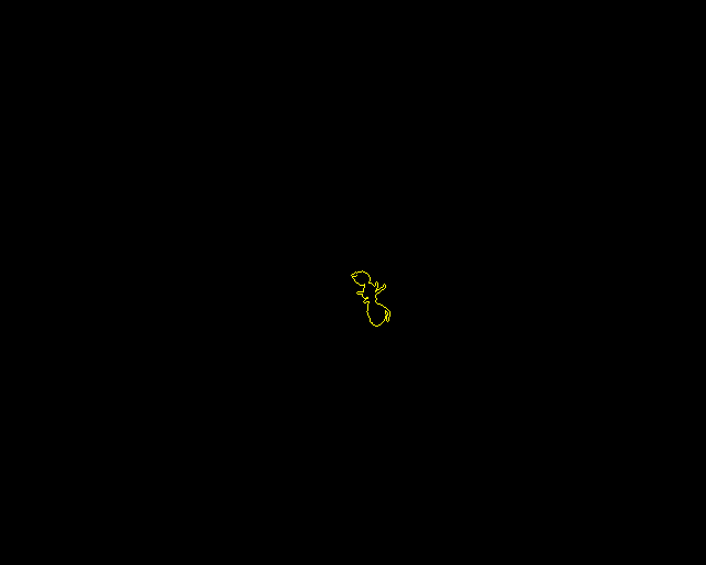
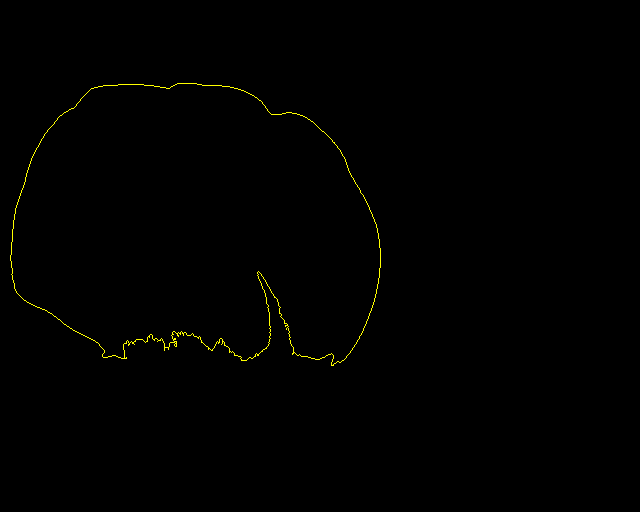
First large contour
Second large contour
Third large contour
Fourth large contour
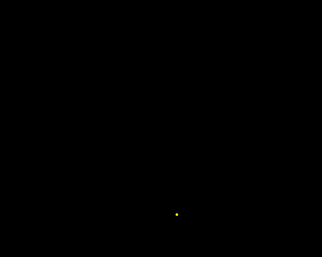
Example tiny contour (first in overall contours list
Figure 4: The four large contours from our example, drawn separately onto a black image, plus the first contour from the original list, drawn on a black image.
1.6 Functions to manipulate contours
OpenCV provides many functions that can manipulate contours; the Structural Analysis and Shape Descriptors documentation page lists many more than we will list here. With these functions we can compute simple geometric figures such as polygons, ellipses, or circles that are close in size to the contour, we can simplify the contour, and we can compute useful statistics such as the area enclosed by the contour.
Mode
Meaning
cv2.drawContour(...)
Draws contours onto an input image with givens color and line
cv2.contourArea(contr)
Returns the number of pixels enclosed by the contour
cv2.boundingRect(contr)
Returns a tuple describing the rectangle that bounds the contour: (upperleftX, upperleftY, width, height) (can draw with cv2.rectangle)
cv2.convexHull(contr)
Returns a new contour that is a convex polygon fitted around the original contour
cv2.fitEllipse(contr)
Returns an ellipse (or a rotated rectangle) that minimizes least-squares error for the contour (can draw with cv2.ellipse)
cv2.minEnclosingCircle(contr)
Returns the center and radius (float values) of the minimum-radius circle that encloses the contour (can draw with cv2.circle)
cv2.minEnclosingTriangle(contr)
Returns the vertices of the minimum-area triangle that encloses the contour (can draw with calls to cv2.line for each pair of vertices)
Each code snippet below illustrates how to call each of the five new functions from the table above, where bc is one of the contours from bigContours above, and fl is a copy of the original peony picture. Figure 5 shows the results of these code snippets on two of the contours.
1.6.1 Bounding rectangle
A bounding rectangle is the smallest rectangle that encloses a certain shape, in this case, a contour. Given a contour, the boundingRect function returns a tuple that describes the bounding rectangle, and which can be passed to cv2.rectangle in place of the two tuples we used before.
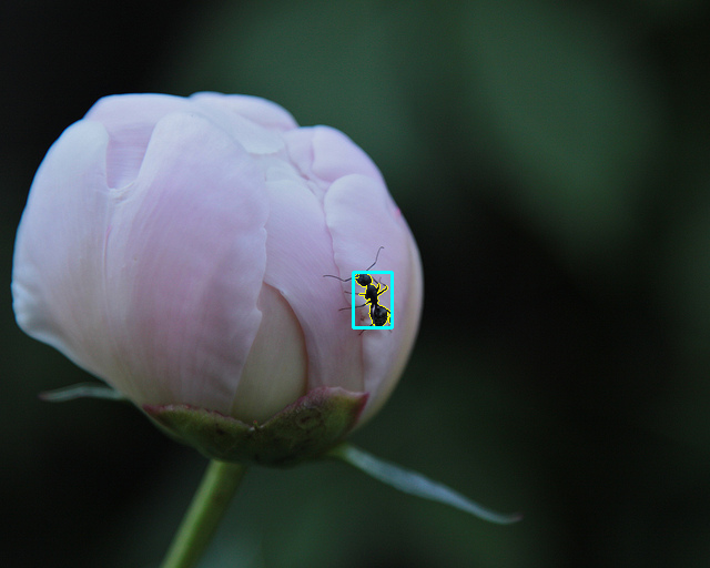
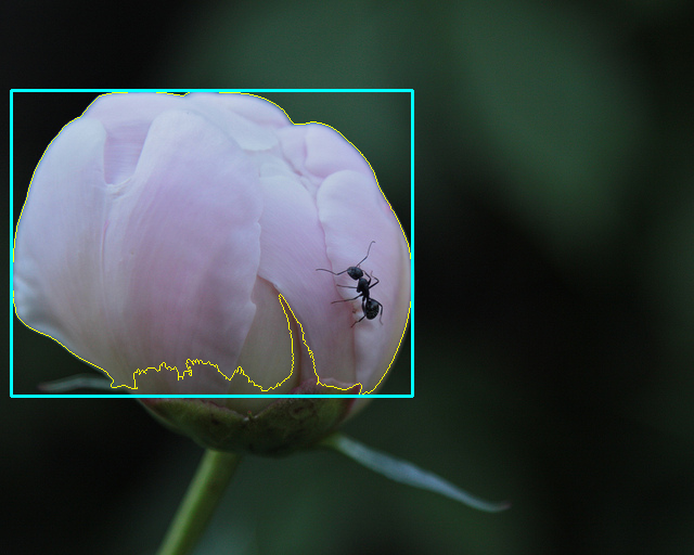
This code first draws just the selected contour on the image, in yellow with one pixel’s thickness. It then computes the bounding rectangle, and draws that on the same image in cyan, with two pixels’ thickness. See the first row of Figure 5 below for two examples.
Besides drawing the shapes so that we can visualize the results, the bounding rectangle might be used to define an ROI that contains a targeted object, or if we were looking for a rectangular object, we could decide if this was it by comparing the area of the contour itself with the area of the rectangle.
1.6.2 Minimum enclosing circle
A minimum enclosing circle is the smallest circle that completely encloses a shape. Given a contour, the minEnclosingCircle function returns a tuple for the circle. The outer tuple contains an inner tuple for the center point of the circle, and a radius for the circle. From this, we could compute the area of the circle or track its position. If we want to visualize it, unfortunately we need to convert the center point and radius to integer values instead of floating-point ones. Then we can use cv2.circle to view the circle that was found.
This code first draws just the selected contour on the image, in yellow with one pixel’s thickness. It then computes the enclosing circle, converts its center and radius to integers, and draws a red circle on the image. See the second row below for two examples.
As for rectangles, we can visualize the circle, but we could also compare its area to the area of the contour to see how round our contour object is, in order to determine whether it is the object we are looking for.
1.6.3 Best-fit ellipse
A best-fit ellipse is an ellipse that best fits the points in the contour. In this case, it computes the least-squares error between the target ellipse and the contour, and minimizes that. In a sense, it is assuming the contour is supposed to describe an ellipse, and producing the best approximation to that ellipse that it can.
This code first draws just the selected contour on the image, in yellow with one pixel’s thickness. It then computes the best-fit ellipse, and draws a blue ellipse on the image. Notice that we can pass the ellipse tuple from fitEllipse directly to the ellipse function to draw it, bypassing all the typical inputs needed to draw an ellipse. See the third row below for examples.
1.6.4 Convex hull
A convex hull is formed using a subset of the points in the contour, but ensuring that they form a convex polygon: a polygon with no indentations in its surface. Imaging stretching a rubber band around the outside of the contour: the points that it touches form the convex hull. Note that the returned value is another contour array: just one that describes a subset of the points from the original.
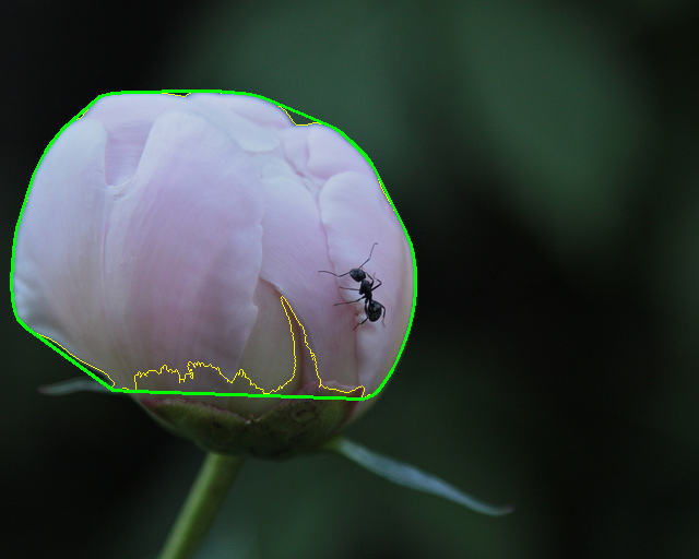
This code first draws just the selected contour on the image, in yellow with one pixel’s thickness. It then computes the convex hull, and draws a green hull contour on the image. The fourth row in Figure 5 below shows examples.
The convex hull is often used to clean up shapes where we have only partially matched the object with our threshold image. It can fill in for missing parts or places where an object is partially hidden by other objects. We can also use it, along with some other functions found on the documentation page, to count and measure the size of the indentations. This can be used to determine, for instance, how many fingers someone is holding up in front of the camera.
1.6.5 Minimum enclosing triangle
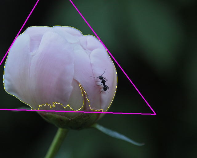
A minimum enclosing triangle is the smallest triangle that completely contains the contour’s points. While less commonly used than the others, this one could be very useful in finding triangular signs, cones, or other triangular shapes. The minEnclosingTriangle function returns the area of the triangle it found, and an array containing three (x, y) coordinates. Because these are all floating-point values, and an interesting structure, it takes a bit of work to extract the values from the returned array, and convert them to integers.
cv2.drawContours(fl, [bc], -1, (0, 255, 255), 1)area, triVerts = cv2.minEnclosingTriangle(bc)[x0, y0] = [int(v) for v in triVerts[0, 0]][x1, y1] = [int(v) for v in triVerts[1, 0]][x2, y2] = [int(v) for v in triVerts[2, 0]]cv2.line(fl, (x0, y0), (x1, y1), (255, 0, 255), 2)cv2.line(fl, (x1, y1), (x2, y2), (255, 0, 255), 2)cv2.line(fl, (x2, y2), (x0, y0), (255, 0, 255), 2)
This code first draws just the selected contour on the image, in yellow with one pixel’s thickness. It then computes the three corners of the triangle, and draws a magenta triangle between them, using the cv2.line function. The last row of Figure 5 shows the result on the ant and peony contours.
1.6.6 Results of drawing shapes for contours
The results below were generated using the code snippets above on the ant and peony contours found earlier.
Bounding rectangle for ant contour
Bounding rectangle for peony contour
Minimum enclosing circle for ant contour
Minimum enclosing circle for peony contour
Best-fit ellipse for ant contour
Best-fit ellipse for peony contour
Convex hull for ant contour
Convex hull for peony contour
Minimum enclosing triangle for ant contour
Minimum enclosing triangle for peony contour
Figure 5: The four large contours from our example, drawn separately onto a black image, plus the first contour from the original list, drawn on a black image.
2 Motion detection and background subtraction
Detecting motion in a video signal is deceptively simple. Making sense of what is moving is much harder, and tracking a moving object is also not trivial. In the first case, we can detect changes from frame to frame in a video signal, and know that whatever is different represents movement in the image. Getting from there to distinguishing between a person moving through a scene, and the movement of trees in the wind, or rippling water, is where things get harder. Separating some movement from the rest and knowing that a particular object is moving takes even more processing.
But we’ll start with the easy step first. The most simple method for detecting motion is simply to take the difference between two frames of an image. The code fragment below illustrates this. Work through what each line does, and then try it out.
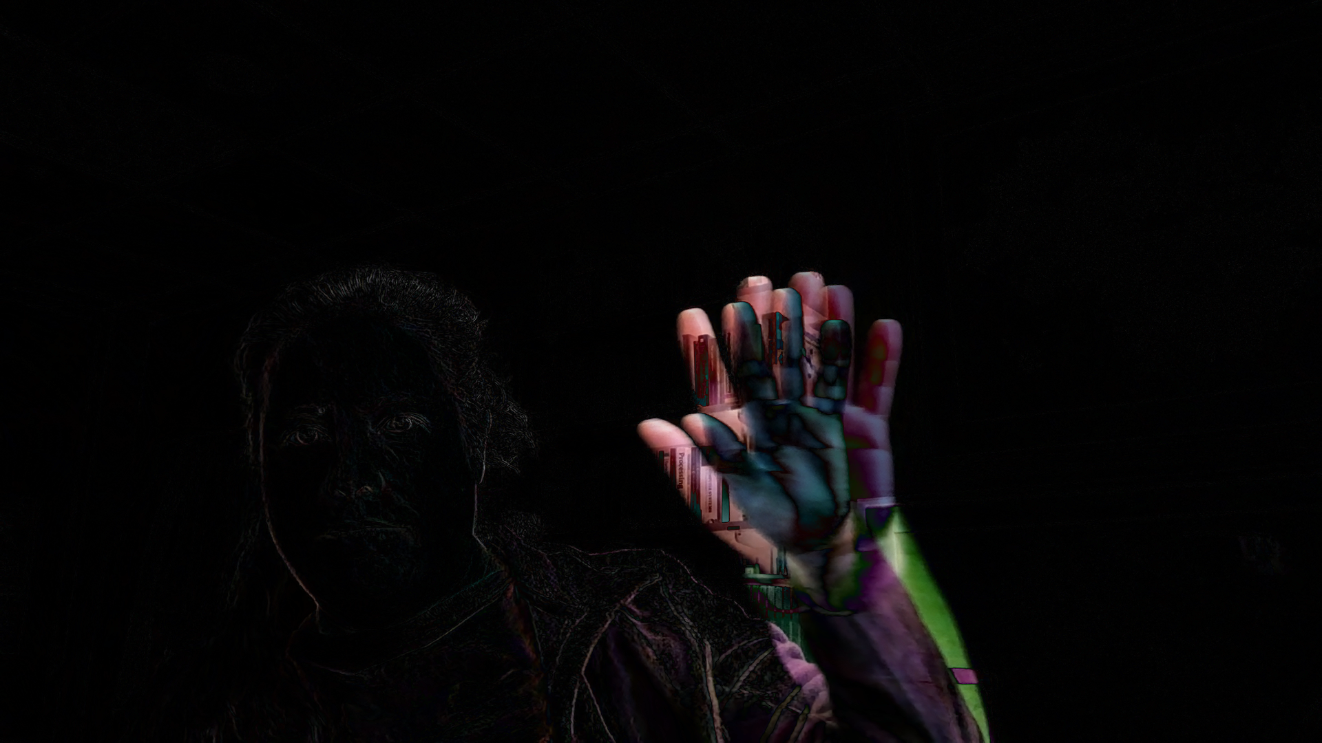
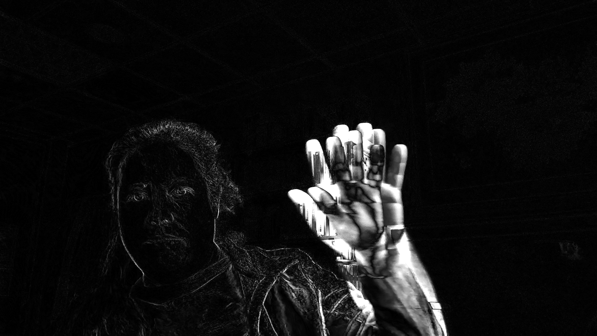
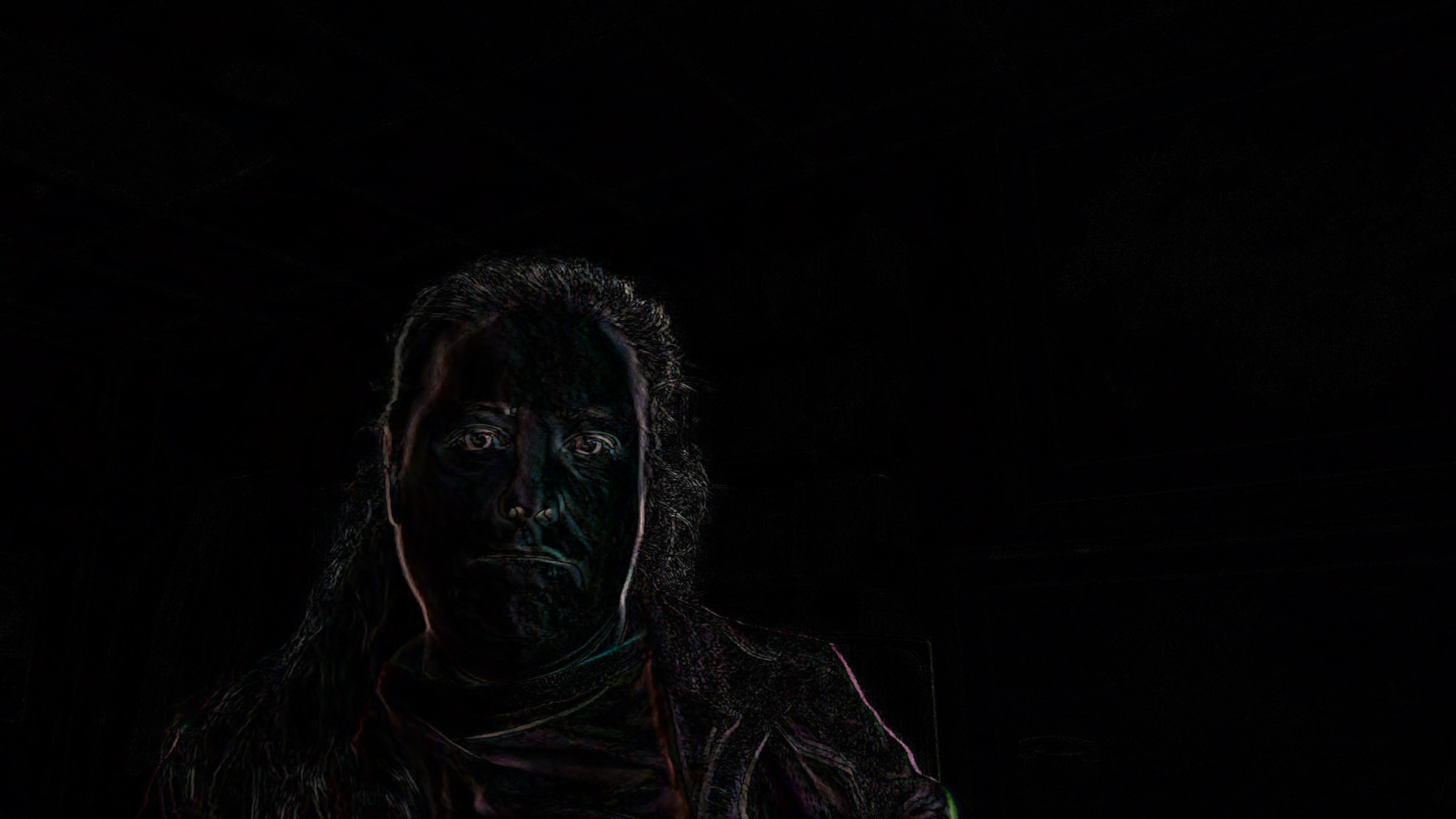
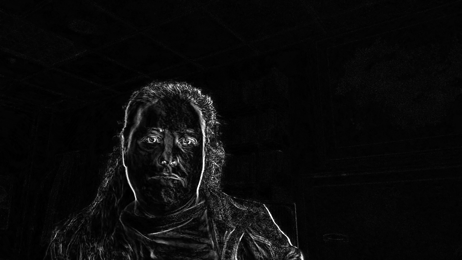
This program computes two forms of the frame difference. The most basic one just computes the absolute value of the difference of the color images, returning a color image. The second form combines the color channels to make one grayscale difference image. Figure 6 shows selected results from this program.
Color absolute difference of frames 1
Grayscale sum of color differences 1
Color absolute difference of frames 3
Grayscale sum of color differences 3
Color absolute difference of frames 2
Grayscale sum of color differences 2
Figure 6: Examples of motion detection through difference of frames, waving a hand, slight movement, and sitting still but blinking
Notice:
The color image shows the impact of the background: where motion is detected you can see a ghostly version of background objects
The color image shows motion less intensively than the gray version, because we add together all three channels
Often only the outer edges of the object in motion are visible, because central parts are still the same color
We can apply thresholding, finding contours, and other techniques to these difference images to locate and identify the movement in a video.
3 Background subtraction
More elaborate methods of separating foreground from background objects exist. The best ones rely on machine learning, which we’ll talk about later on. But there are several algorithmic approaches.
They all have a similar form:
Given a sequence of frames from a video, construct a “model” of the background of the space (based on which pixels do not change much in brightness or color).
For a new frame of the video, compute the difference between the background frame and the new frame.
Build a mask image of the pixels that are significantly different from the background: these mark the location of the foreground object
Apply the mask to the new frame and display the results
What changes between different methods is how we build or calculate the background model.
3.1 A simple attempt at background subtraction
The simplest approach is to take a picture without the foreground object in it, and just use that for the model. This has only mediocre results.
The code sample below uses this method to produce a masked version of the original video feed with the background set to black. It first loops on the video feed, until the user hits q. At that point, the last frame read is set up as the background picture. A more elaborate implementation would perhaps read multiple frames and average them together to form the background image.
capture = cv2.VideoCapture(0)capture = cv2.VideoCapture(0)# Get the background as a single frameprint("Press q when ready to take background picture")whileTrue: gotIm, frame = capture.read()ifnot gotIm:break cv2.imshow("Frame", frame) x = cv2.waitKey(10)if x >0andchr(x) =='q':breakbackgroundPic = frame
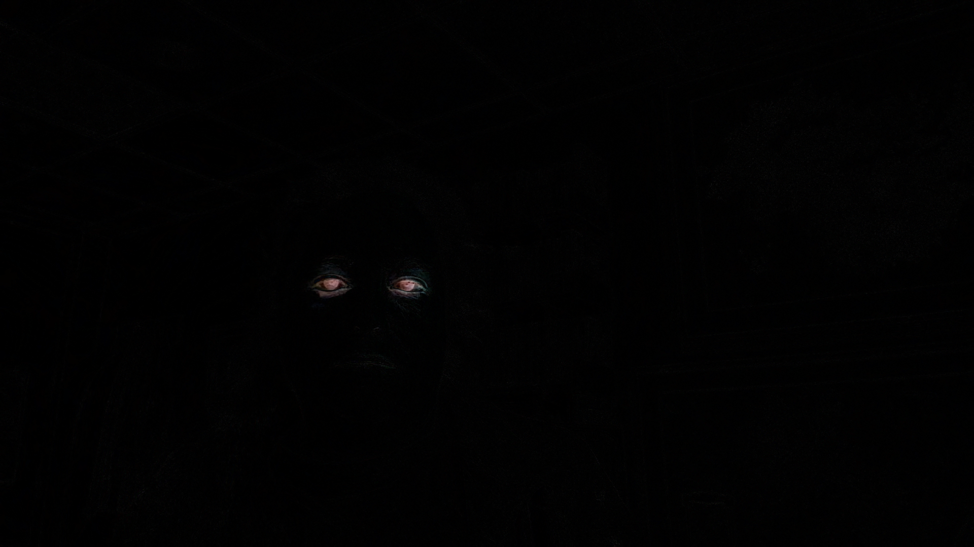
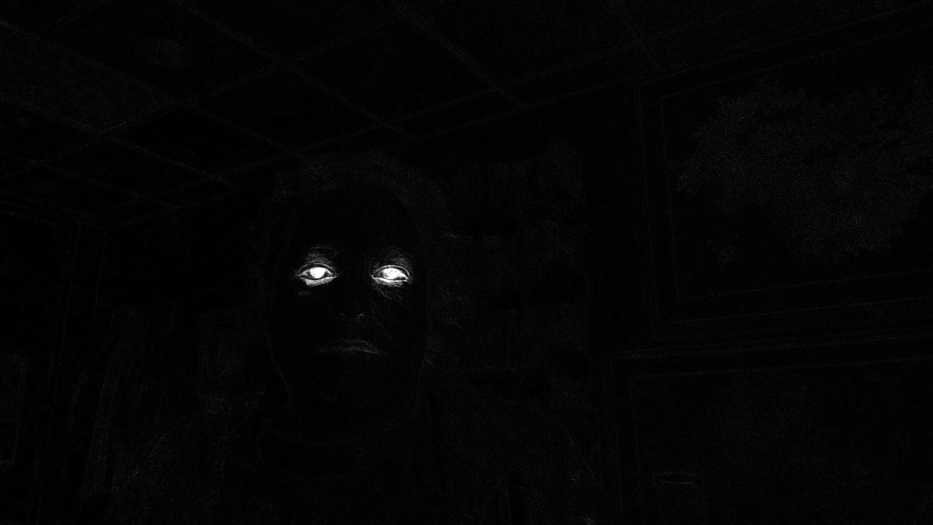
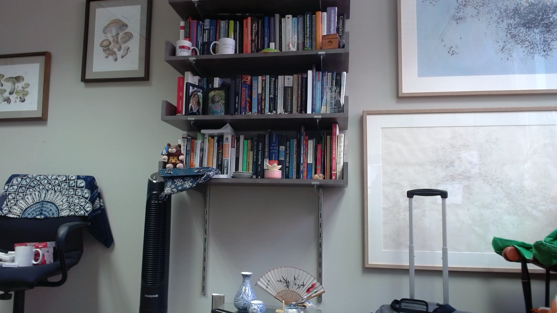
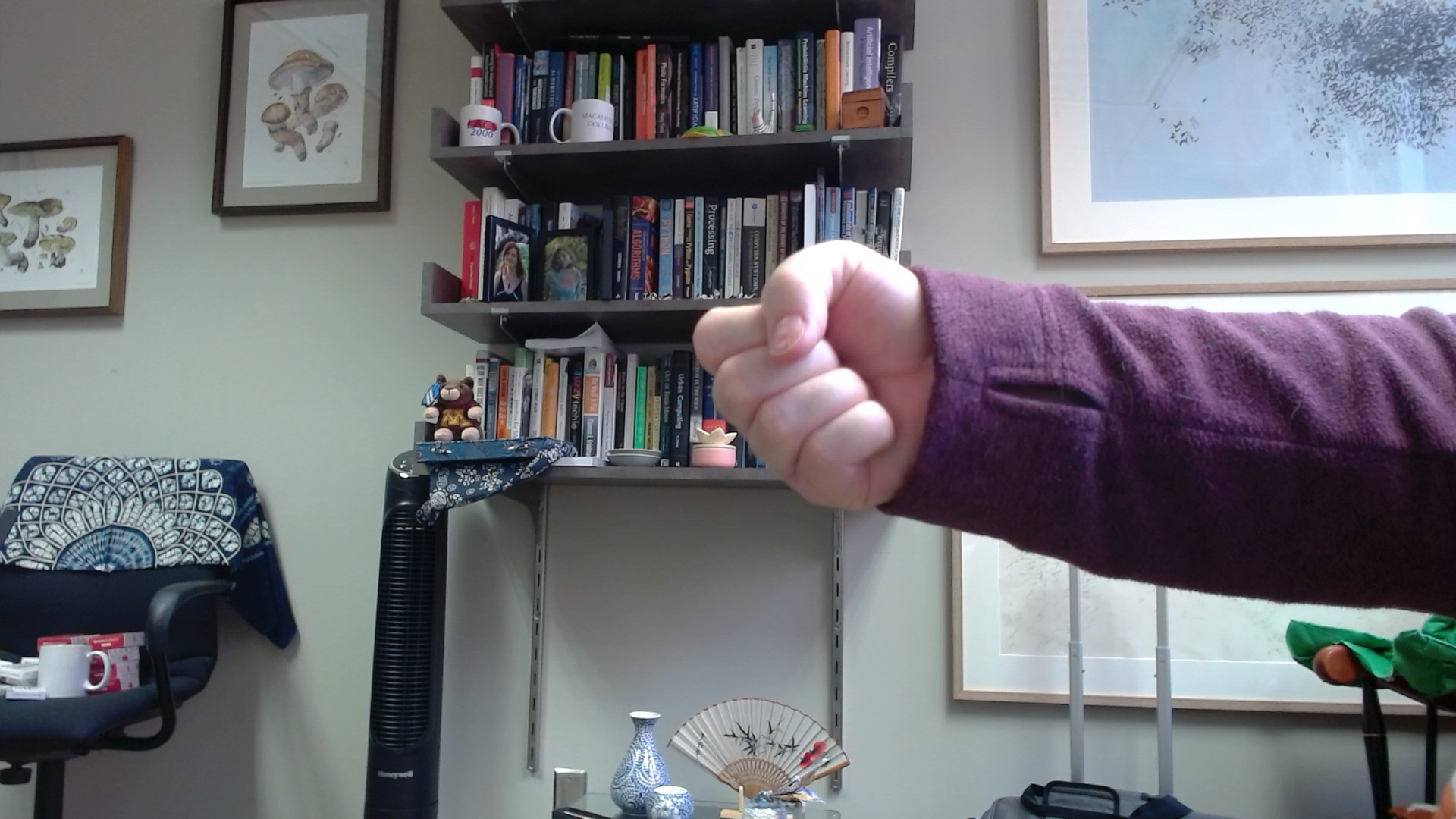
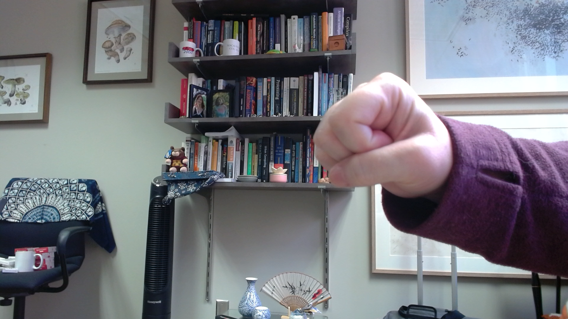
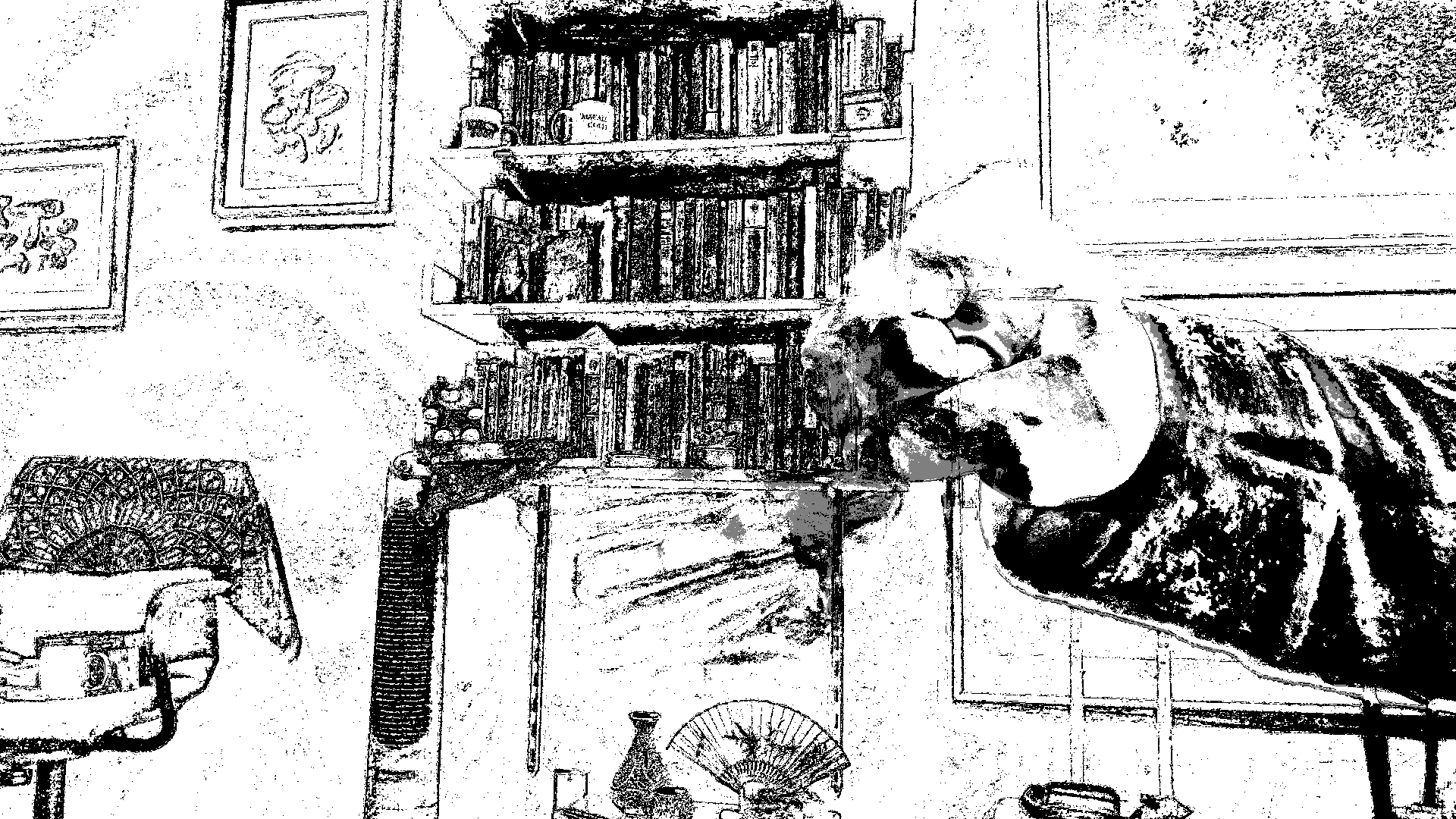
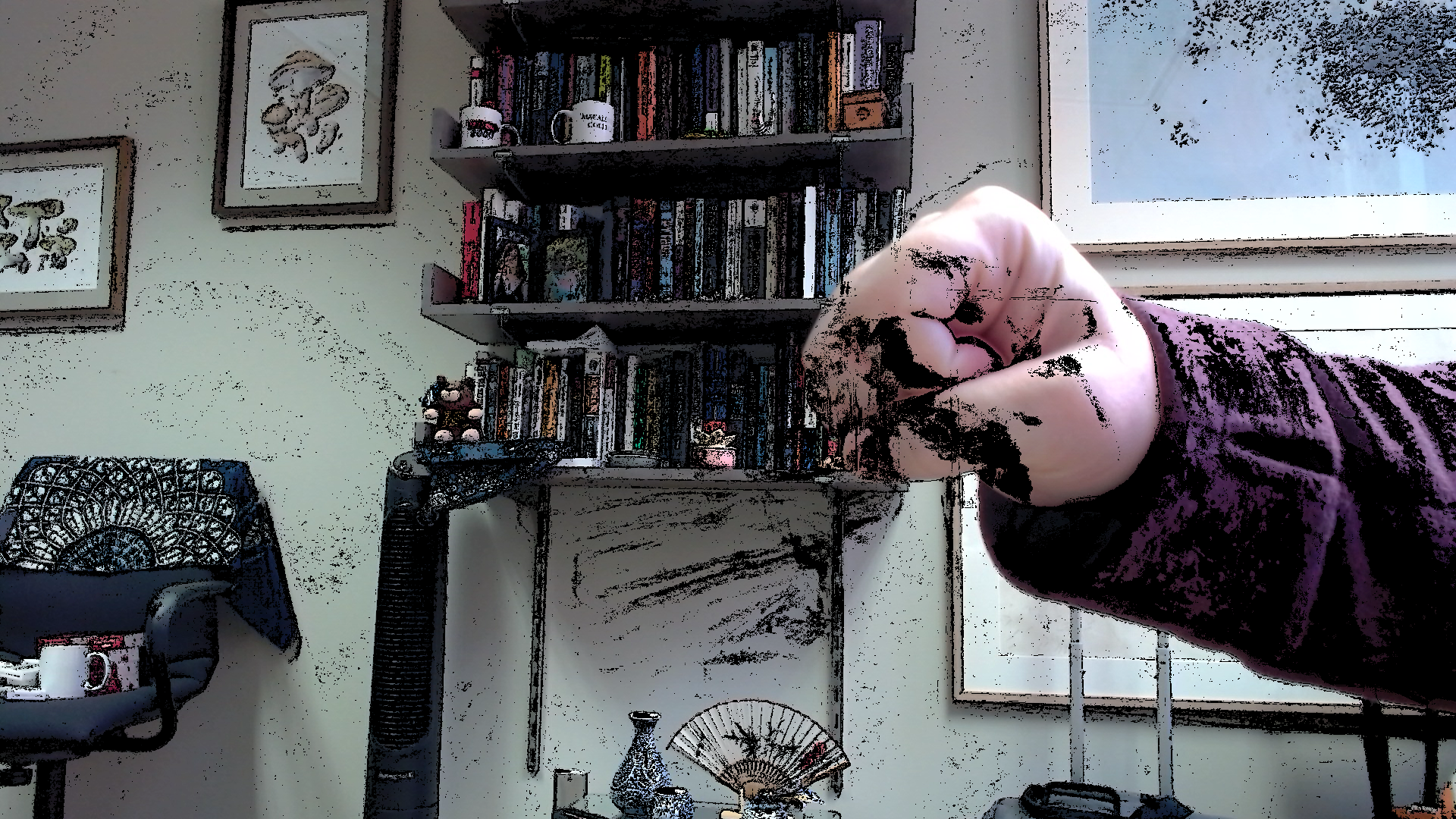
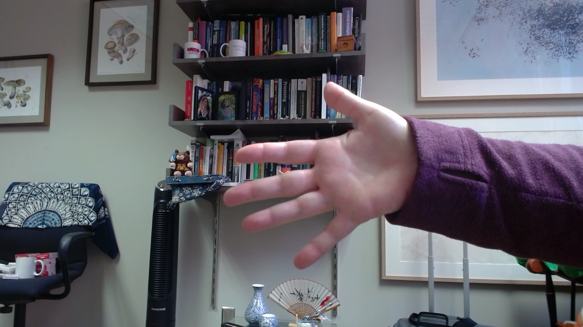
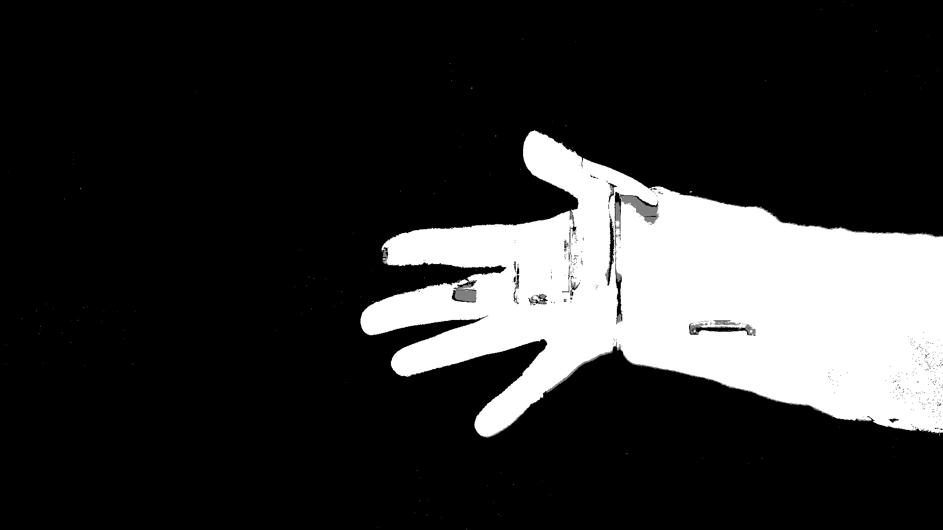
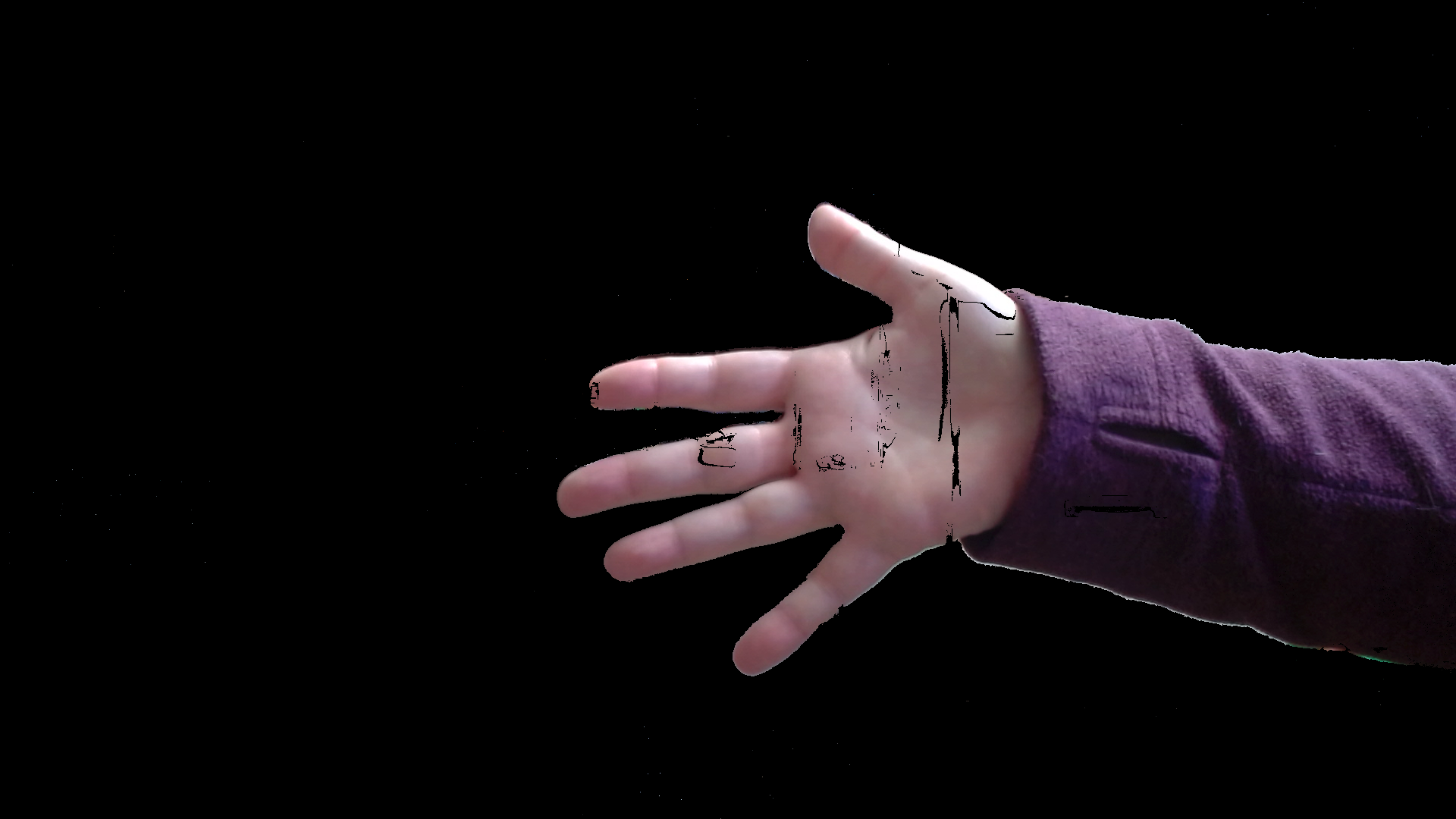
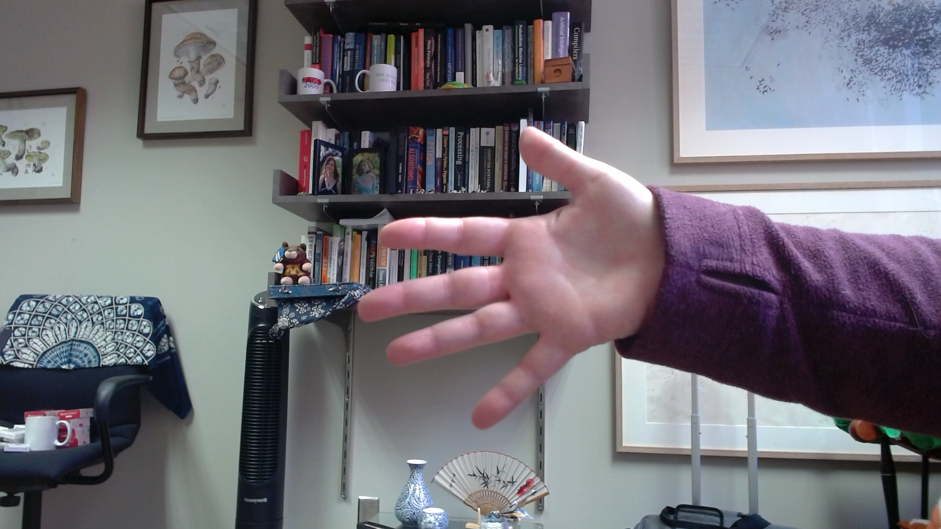
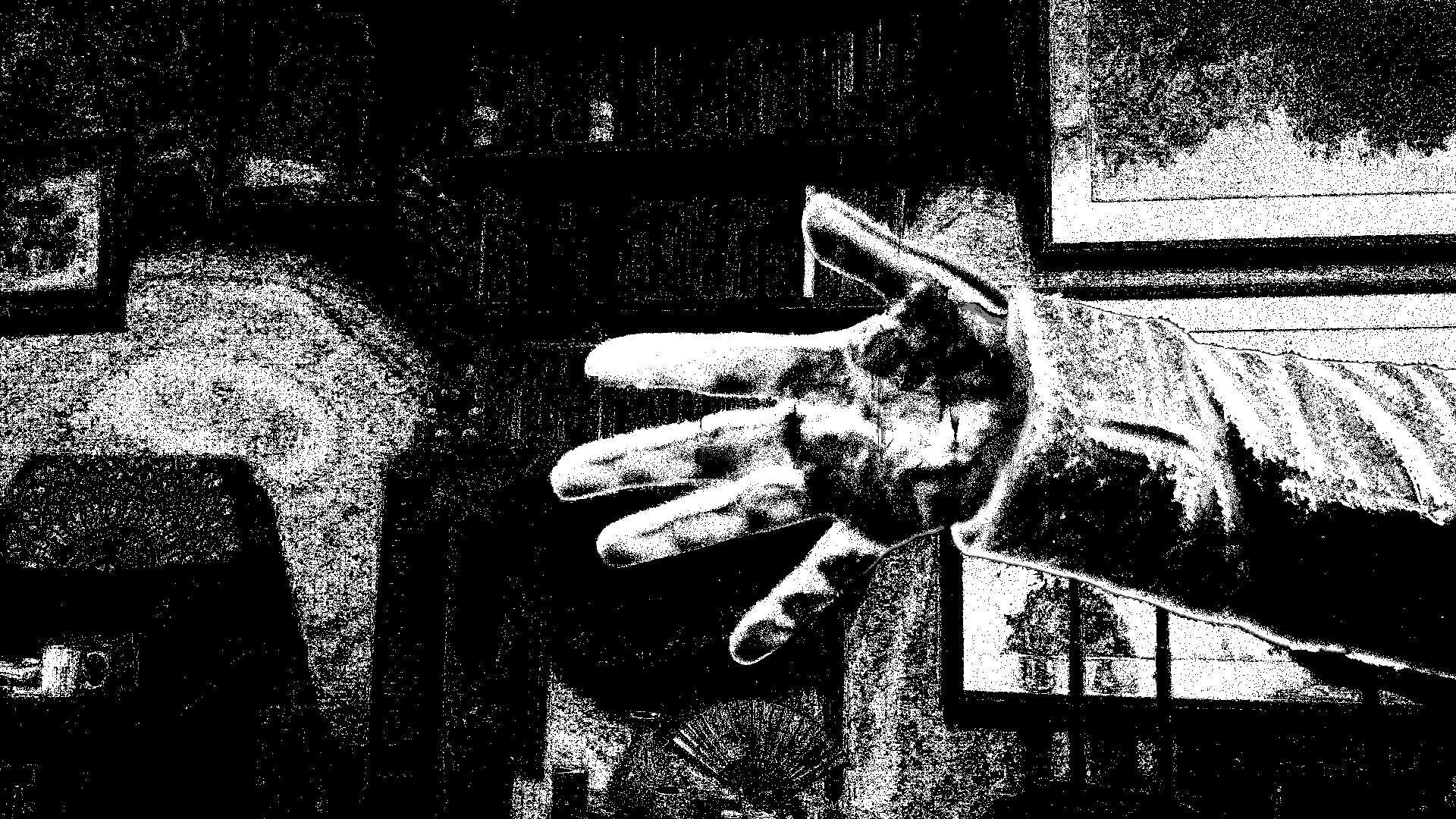
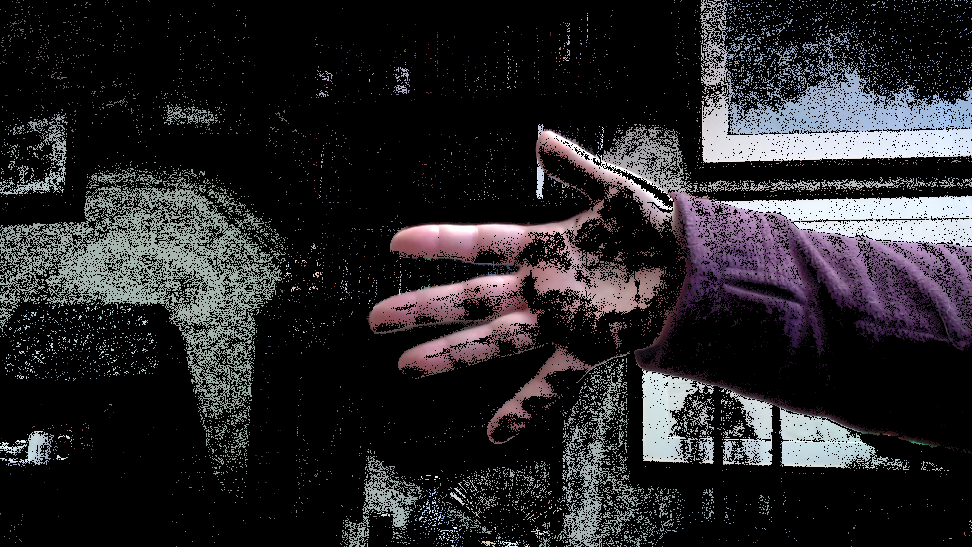
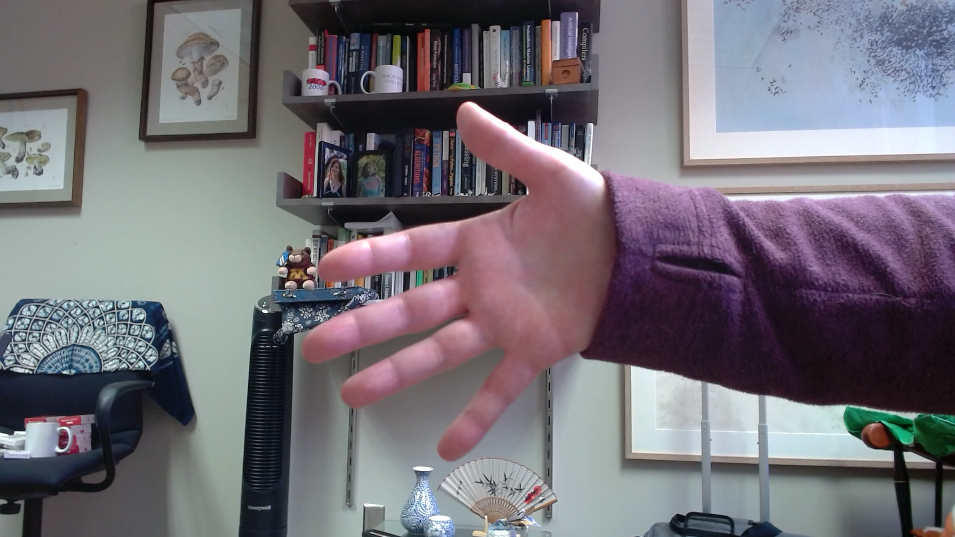
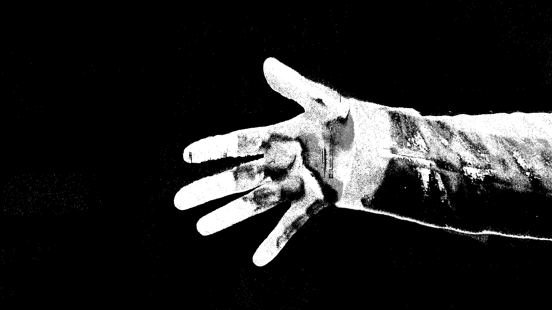
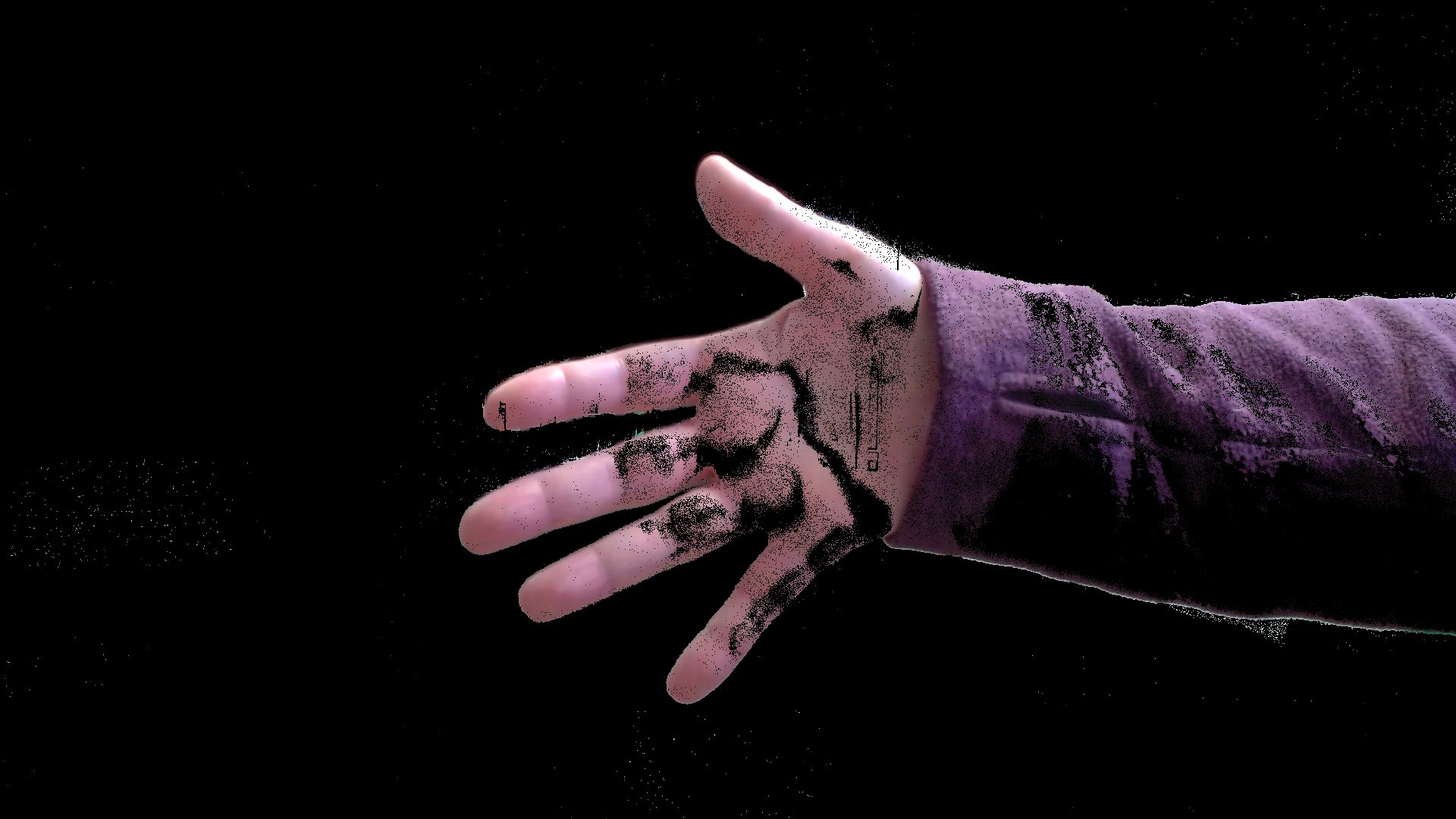
After setting up the background image, the program continues in the next code sample. For each frame, it computes the difference from the background picture, and then combines the color channels together. In this case we average them together, instead of adding them as we did for motion detection above. Finally, we use a threshold to turn the difference image into a black-and-white mask, and we apply it to the frame to get just the foreground. Figure 7 shows the background image, the foreground image, and the result of our attempt at background subtraction.
Figure 7: The background picture, foreground (unprocessed frame), and the result of applying the simple background subtraction. Note that the pattern showing on the hand is due to the books on the bookcase matching the hand color too well.
3.2 The MOG (Mixture of Gaussians) approach to background subtraction
OpenCV provides an implementation of an algorithm commonly calls “mixture of gaussians.” With this, we build a more complex model of the background of an image. By looking at a selection of recent video frames, the model starts with a range of values for each pixel in the background. They then characterize the range for each pixel as the combination, the mixture, of several gaussian functions. These allow the model to capture complex variations (like sudden brightening in one area caused by wind shifting tree branches, for example).
The code sample below shows how to set up and use the MOG-based background subtraction method. Figure 8 shows the original frame and the masked result for this method.
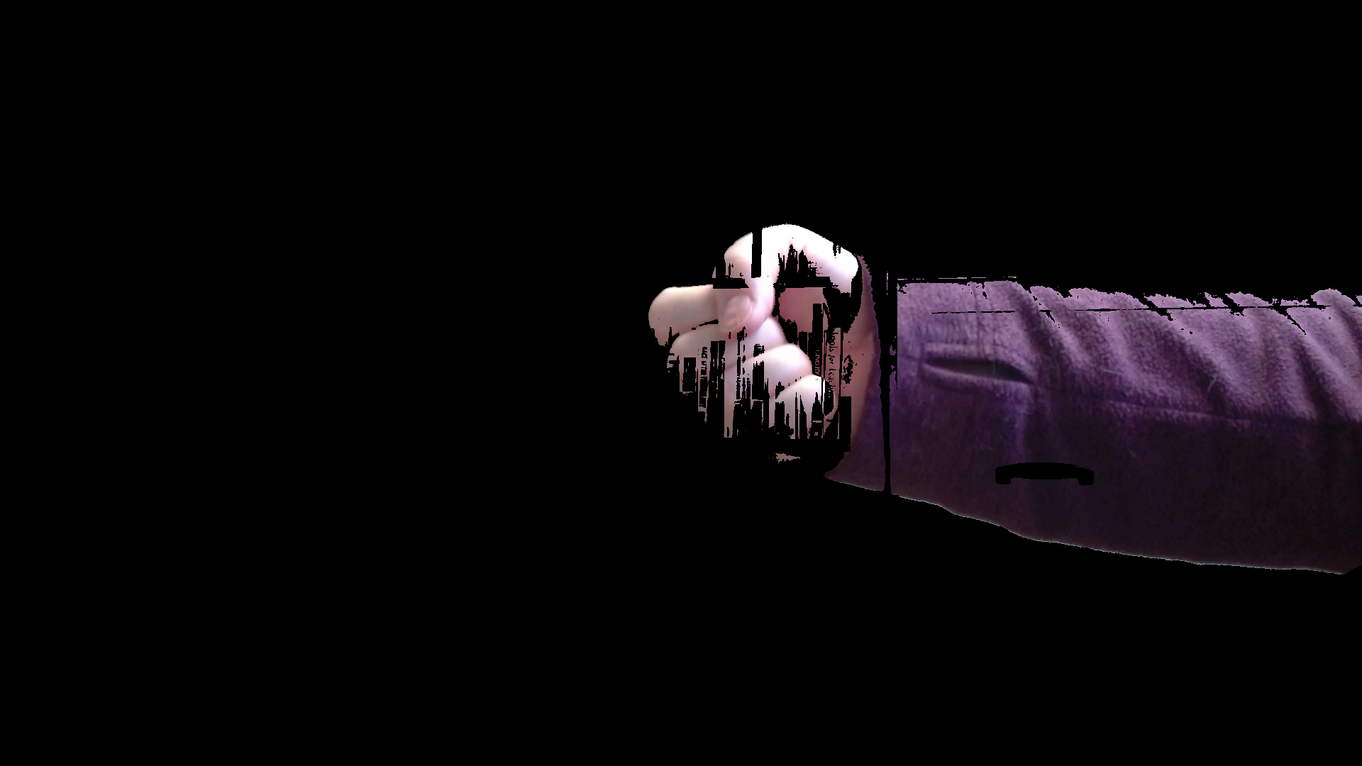
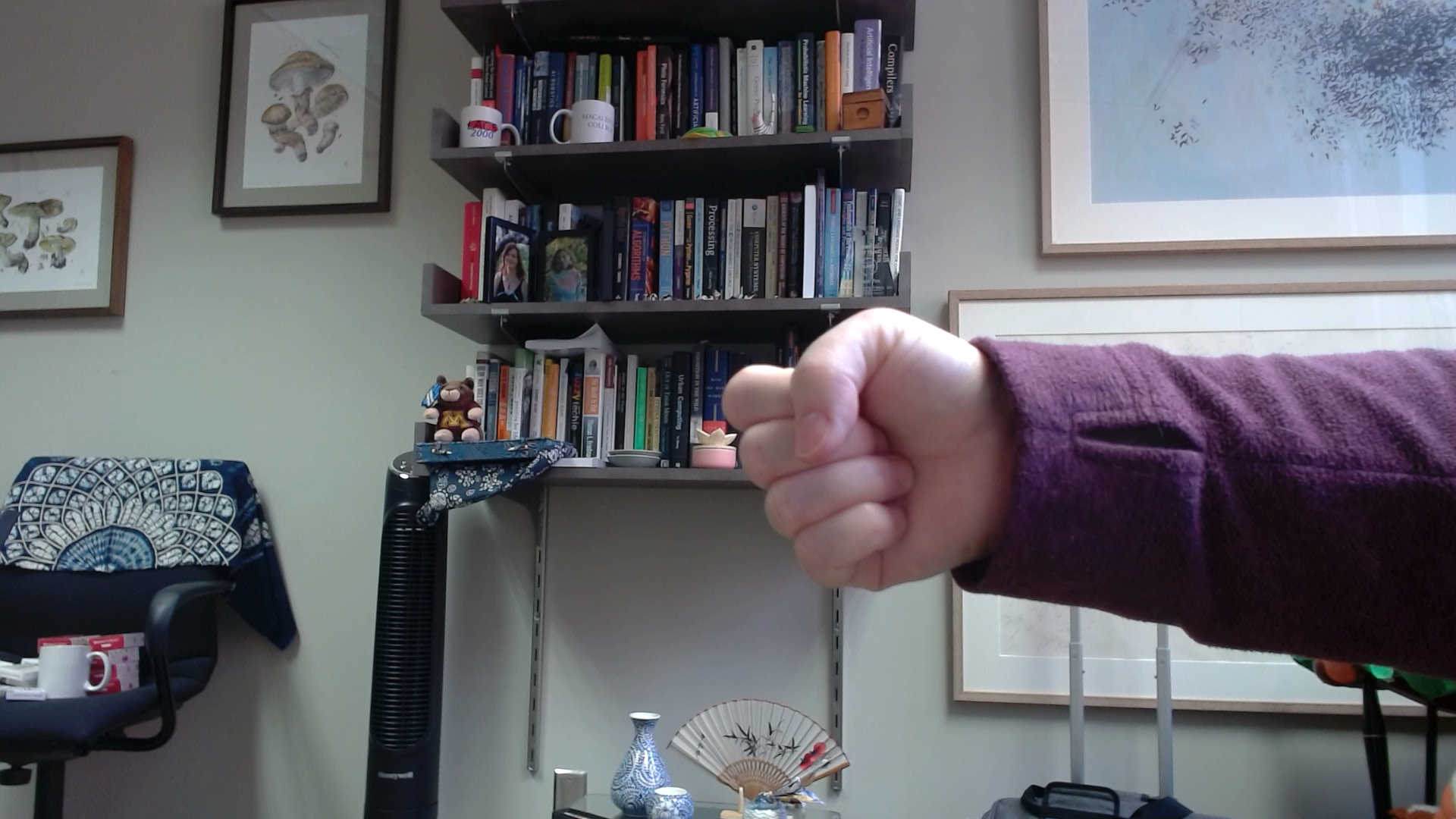
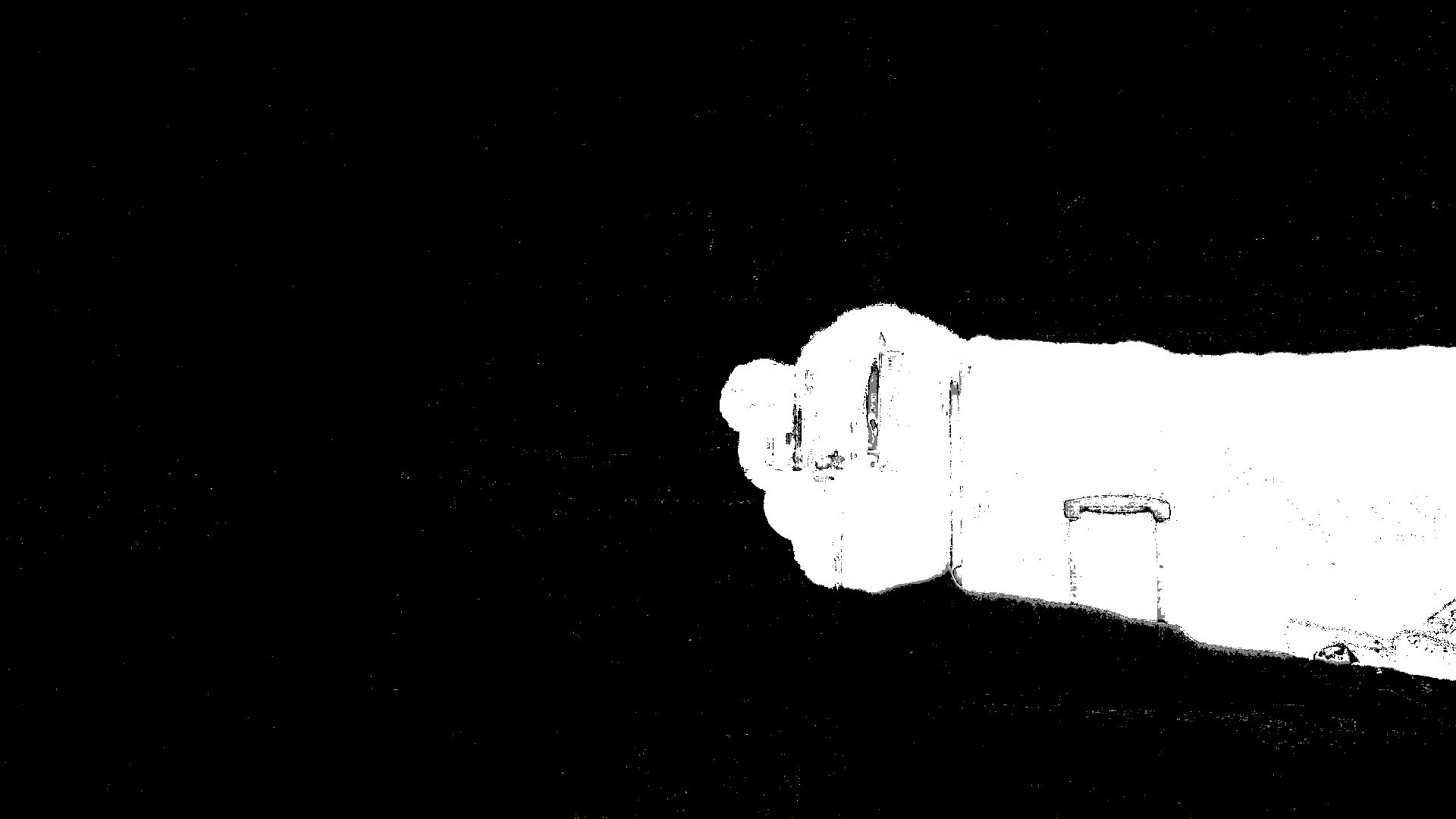
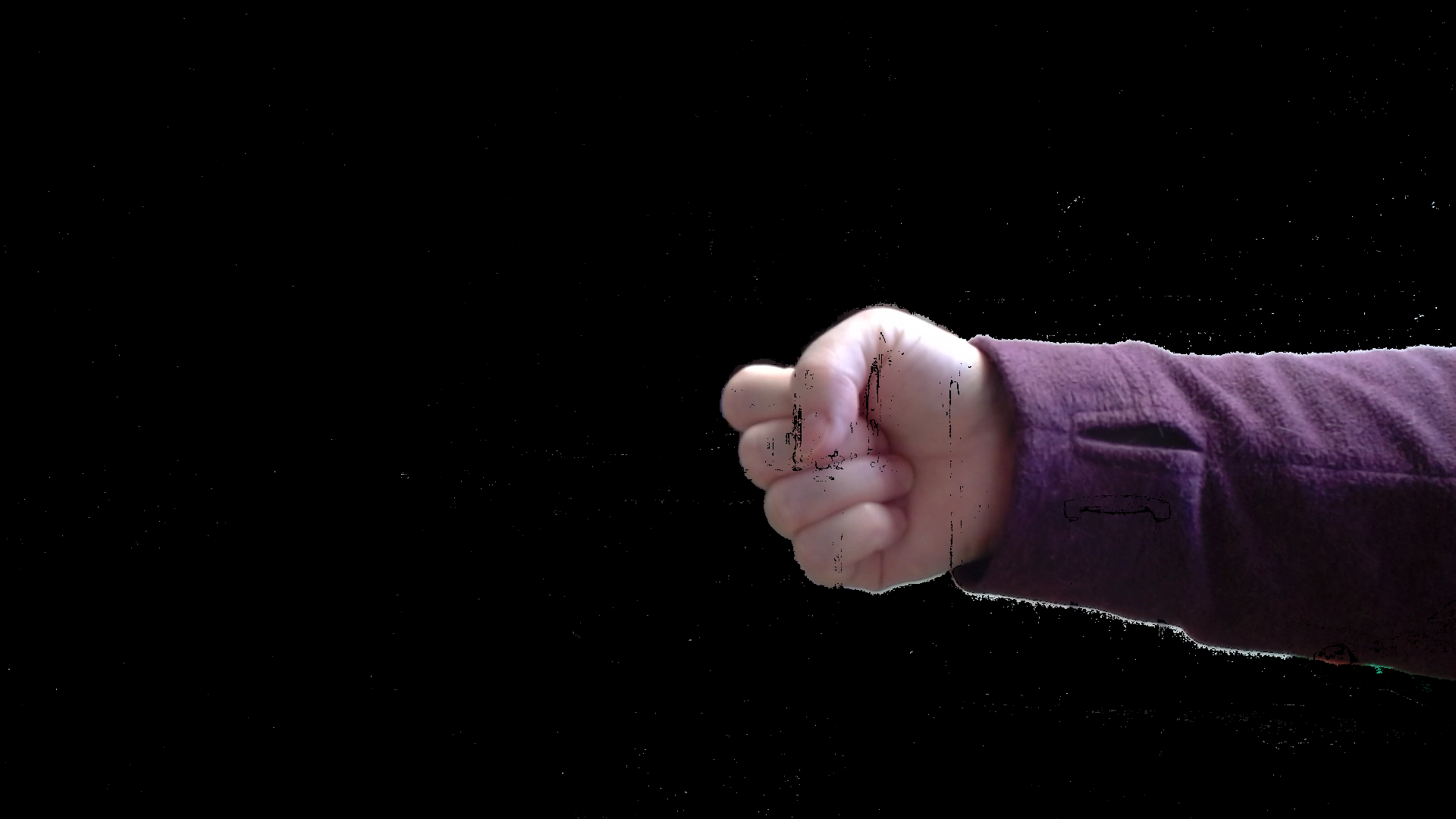
The first set of photos in Figure 8 illustrate the ideal operation of the algorithm. After letting the background sit empty for a few seconds, I then moved my arm into view. The algorithm accurately identified my arm as “foreground” and constructed a mask that correctly removed the background pixels. However, I then held my arm still in view for a few seconds. This was long enough for my arm to become incorporated as part of the background, so when I started to move my arm, the algorithm became confused overall, and failed to subtract the background properly.
Foreground when arm first moved into view
Mask created by MOG when arm first moved into view
Final result when arm first moved into view
Foreground after arm stationary for a few seconds
Mask created by MOG after arm stationary for a few seconds
Final result after arm stationary for a few seconds
Figure 8: The original frame, the mask created from it by the MOG algorithm, and the final masked result, shown at two times: just after the arm moves into view, and after the arm is stationary for a few seconds.
3.3 The KNN (K-nearest neighbor) approach to background subtraction
The KNN backgroung subtraction algorithm defines a sphere for each pixel. The dimensions of the sphere are the BGR values (color channels). The size of the sphere is chosen dynamically so that it encloses K of the previous frames’ colors at that pixel. You can change K to tune this algorithm. For a new frame, if the color at a pixel falls within the sphere defined for that location, then it is categorized as a background pixel, and if it falls outside of it, then it is categorized as a foreground pixel. Much like the previous algorithm, what count as background is updated dynamically to accound for lighting changes that happen gradually over time.
The code sample below shows how to set up and use the KNN-based background subtraction method. Figure 9 shows the original frame and the masked result for this method.
Figure 9 shows the result after allowing the algorithm to see the background for a few seconds, and then moving my hand into the frame. After just a few seconds of holding still, the algorithm destabilizes. However, the KNN approach improves the longer it runs, so the third row illustrates what happens after a long time with me moving my hand in and out of view. The algorithm has re-stabilized to identify my hand better.
Foreground when arm first moved into view
Mask created by KNN when arm first moved into view
Final result when arm first moved into view
Foreground a few seconds later, when I move my arm
Mask created by KNN a few seconds later
Final result a few seconds later
Foreground after a longer run, with arm stationary for several seconds
Mask created by KNN at that later point
Final result at that later point
Figure 9: The original frame, the mask created from it by the MOG algorithm, and the final masked result, shown at three times: after just a few seconds of background when arm moves into view, after a few more seconds, when the arm moves again, and after 10-15 seconds of run time, with a stationary arm in view.
A Medium blog by Isaac Berrios does a nice job of showing how these algorithms work on a better use case: surveillance of a road. In that case, moving objects are the focus, and they will keep moving. If a car pulled over to the side of the road, however, it would disappear to become background fairly rapidly.
4 Color-tracking with CAMShift
The previous methods looked for objects by their motion against a static background. In this approach, we will look at tracking an object by its color, in a way that is robust to some changes in lighting.
When we track an object as opposed to detecting an object, we keep track of its position from one frame to another rather than finding it from scratch each frame. Our previous work only detected objects, it did not take the extra step to track them. CAMshift does tracking, and it is an important part of the algorithm’s workings.
Color is a highly salient feature of objects in the world, and useful for tracking an object in a video signal. That said, color can vary depending on how much light, and what color of light, is lighting a scene. The technique shown here works relatively well in neutral light conditions, within a reasonable range of ambient light.
CAMShift stands for “Continuously Adjusting MeanShift.” So first we’ll talk about what MeanShift does, and then what CAMShift does differently. Note that both MeanShift and CAMShift are implemented by OpenCV. Meanshift is a technique that originates in statistics, as a way of analyzing a distribution of data. It just happens to apply to images under certain circumstances.
Both these algorithms are built on the same underlying calculations about tracking a color or colors. Given a frame of a video, we want to compute which pixels match the colors we’re tracking, and how well they match. The section on “Histograms and Backprojection” below revisits the idea of backprojection from an earlier chapter. What we have, in the end, is a grayscale “image” where the brightness of each pixel represents how well the corresponding pixel in the frame matches our target colors. We call this the backprojection.
The backprojection is then used by MeanShift and CAMShift to find the central object of the target color. MeanShift moves a fixed-size tracking box around the backprojection to find the region that is most dense with the target color, and where the pixels are the strongest matches to the target color. CAMShift adjusts the size of the tracking box each time through to match the density of the backprojection.
4.1 Histograms and Backprojection
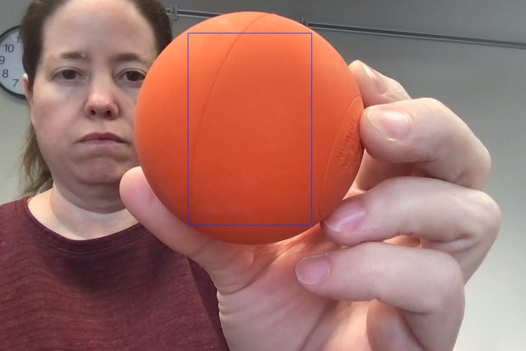
These algorithms use the HSV color format, and construct a histogram of hues (colors) that are the targets. The histogram is constructed by providing or selecting a reference image, either a whole image or a region of interest where all the pixels are the target colors. The example picture in Figure 10 shows a region of interest in the overall picture that includes only the orange ball. We will use this region to build the histogram.
Figure 10: Picture of orange ball with ROI for histogram marked by blue rectangle
To build the histogram, we:
Convert the image to HSV
Threshold/mask away pixels that have low saturation or low value (because very dark pixels tend to have nearly random hues assigned, so they are unreliable and noisy)
Use only the resulting hue channel
Have OpenCV build a histogram of the values in the hue channel
A histogram has a set of bins, and the value in each bin represents how many instances had a value in the range of that bin. Hue values will always be an integer between 0 and 179. So if we chose to have 10 bins, then all hue values between 0 and 17, inclusive, would map to the first bin; all the values between 18 and 35 would map to the second bin, and so forth.
For this application, we usually choose 16 or 32 bins, for no particularly good reason.
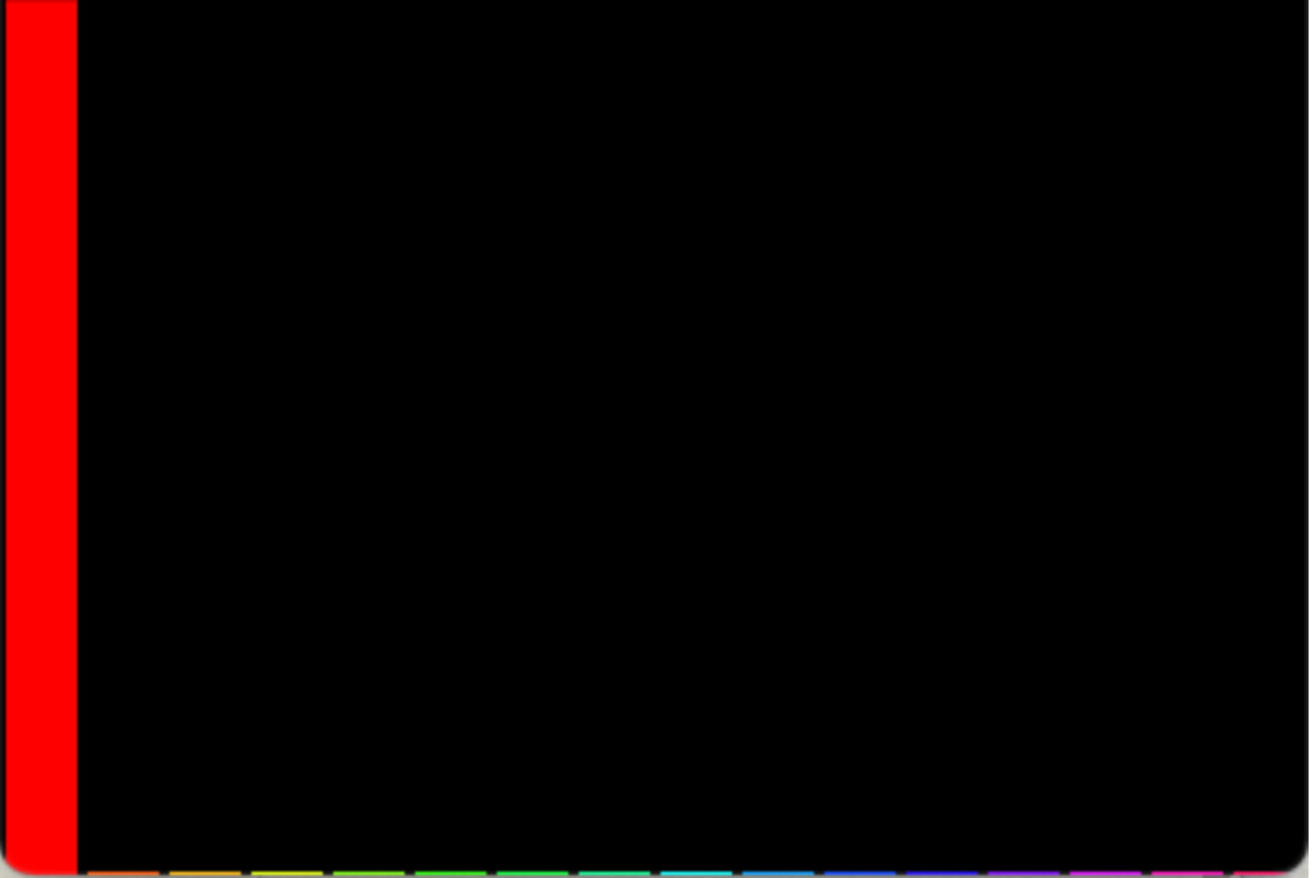
Thus, the value in each bin of the histogram records how many pixels are within each range of hues in the target color image. Often the histogram emphasizes a single narrow range of hues, but you could also track a blue and green object with a histogram that contains both blue and green. Figure 11 is a view of the histogram that would result from the region of interest shown above.
Figure 11: Histogram for orange ball colors selected earlier
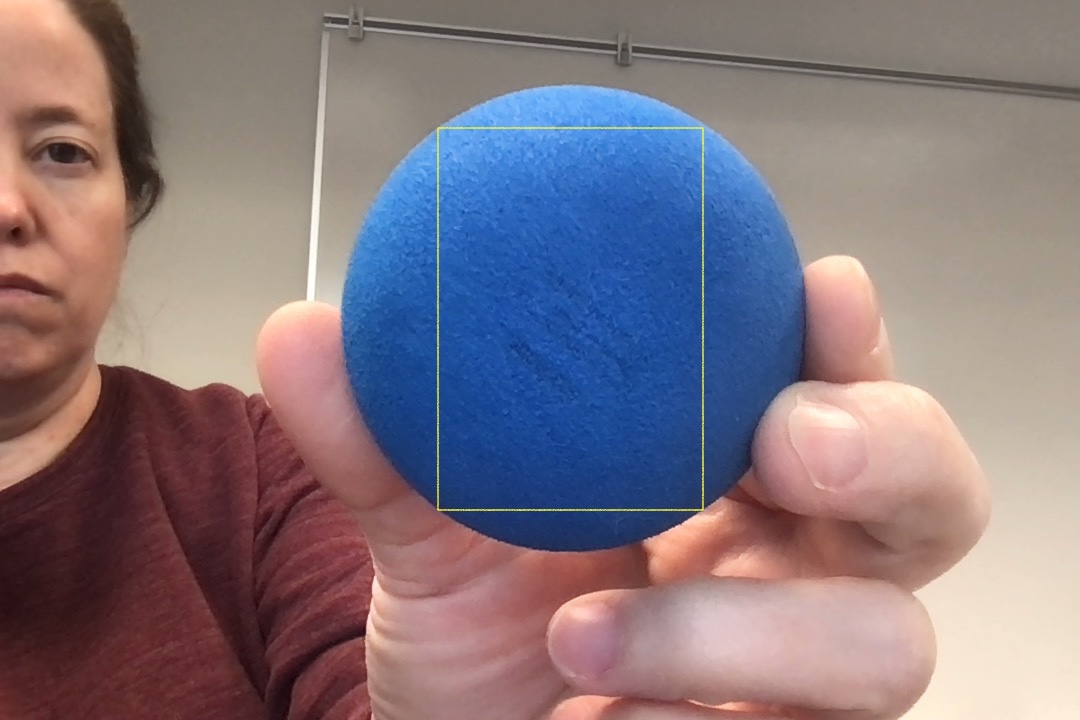
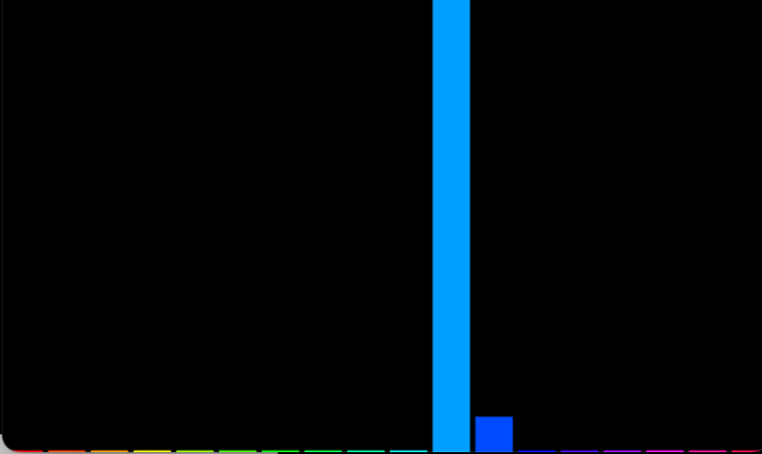
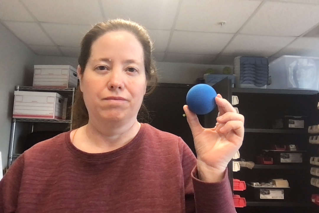
And Figure 12 shows another example of the histogram for a different color:
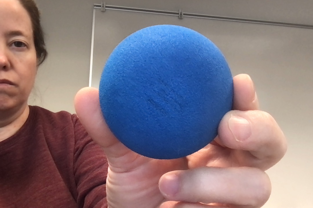
A picture with a blue ball with the ROI for its histogram marked by a yellow rectangle
Blue histogram built from the previous ROI
Figure 12: A picture of a blue ball, with a suitable color ROI selected, and the hue histogram that would result.
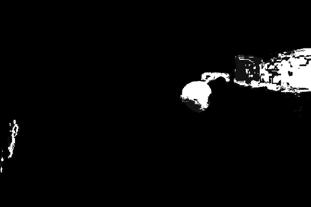
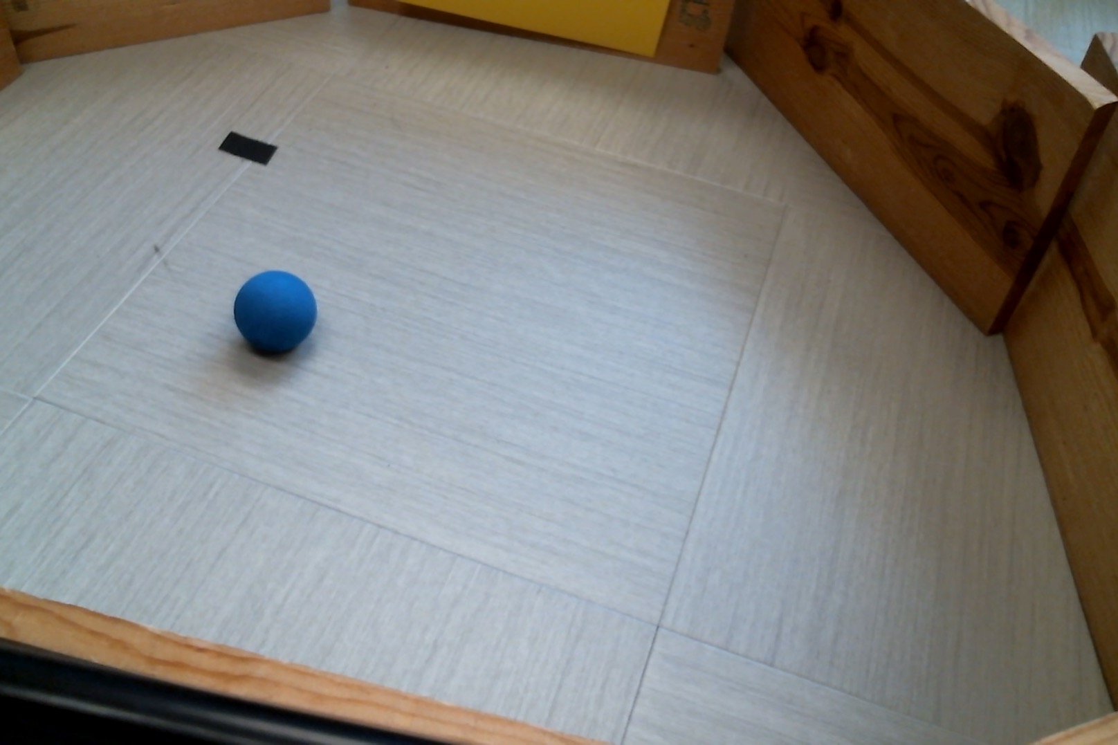
When we want to find the target color/object in the video stream, we take a frame from the video, and extract its HSV Hue channel. Then for each pixel we compute the likelihood that its color is the target color, using the height of the bars in the histogram for that particular hue. This likelihood is stored as a grayscale “image” where strong matches are brighter than dim matches. This is called the backprojection, or backproject, of the frame.
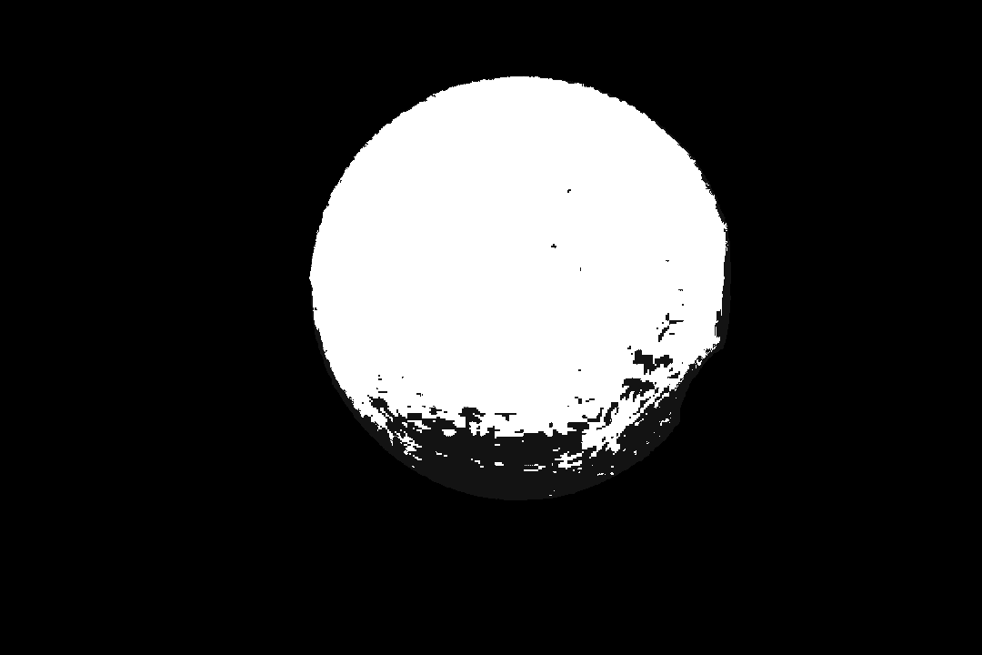
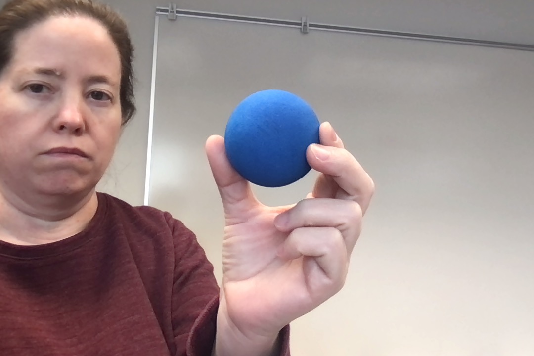
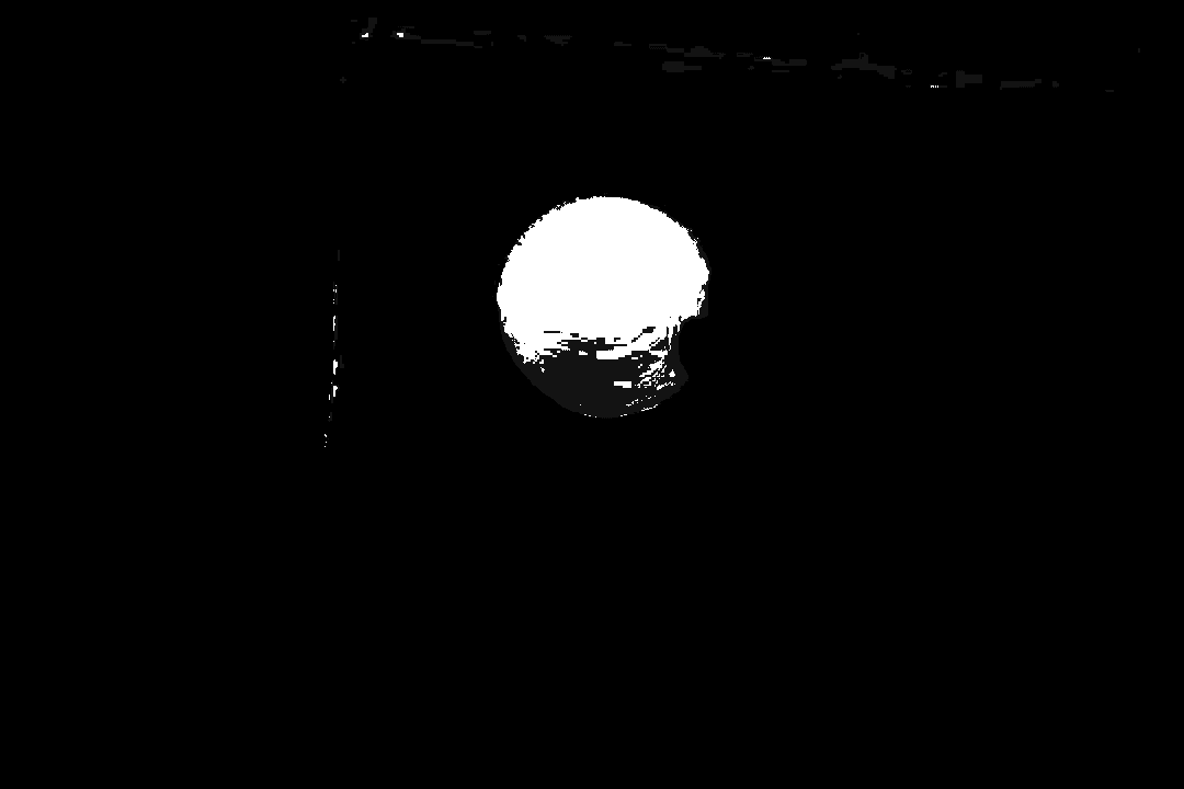
#fig-backprojs shows four blue images, and the backprojections we get when applying the histogram above to each image. Some find the ball strongly, others less well because of other objects or very different lighting conditions.
Original image with ROI for reference image
Backproject for original blue image
Similar image with blue ball
Backproject for second image
Similar image with different background
Backproject for third image
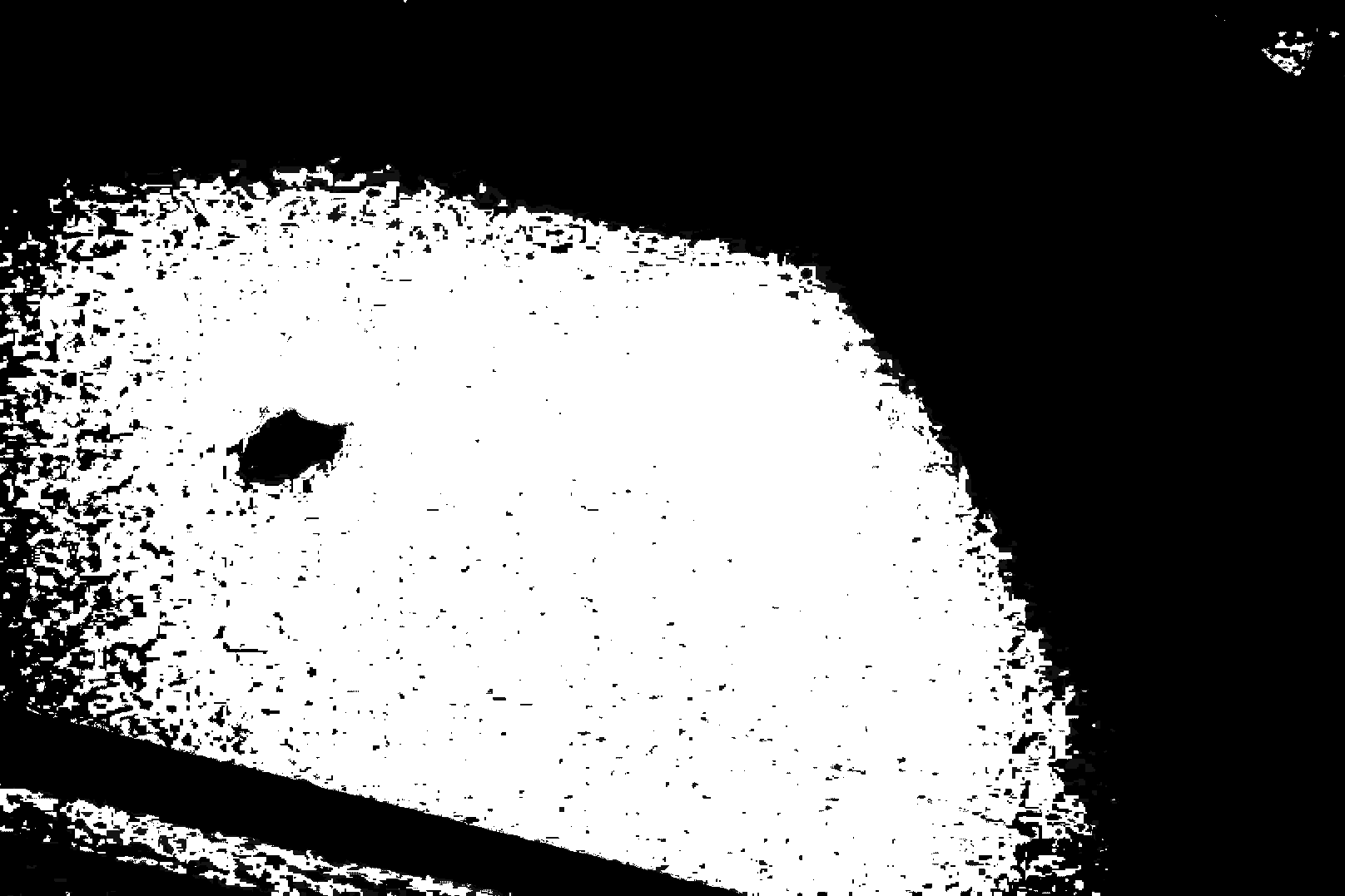
Same ball in different context
Backproject for fourth image
Figure 13: Various back projections with different ball positions and lighting
The last example in Figure 13 illustrates the limitations of color-tracking. Because the floor has a blue-ish tint to it, the blue ball is lost in a seat of other pixels that match the color well enough. We would have to perform some preprocessing to isolate the ball in this context.
4.2 The MeanShift algorithm
MeanShift is an algorithm used beyond computer vision; it is sometimes used in statistics or probability calculations as well. I’m just going to describe it in terms of computer vision. MeanShift takes the backproject of an image, and it starts with a fixed-size rectangular track window that is placed at some location in the image. The first time it is run, the track window may be placed in any location. On subsequent runs, the track window starts where it ended after the last run.
MeanShift computes the center of mass of the backproject values in its track window. That basically means the location, taking into account the backproject values as weights, where there is an equal amount of weight in every direction. Imagine that the track window of the backproject is a flat platter, where the thickness at each point corresponds to the backproject value. The center of mass is the point where you could balance the flat platter on top of a pin.
If the center of mass is located at the center of the track window, then the algorithm ends and reports the window’s current position. If the center of mass is not at the center, then MeanShift moves its track window to be centered on the center-of-mass, and then repeats the process, from the step where it computed the center of mass. It repeats this process of moving the track window until either some maximum number of iterations occurs, or the center of mass is at the center of the window. The pseudocode below captures the main points of MeanShift
Algorithm meanShift(backProjImage, oldTrackWindow)
1. Repeat at most N times
2.     Let cm be the center of mass within oldTrackWindow of backProjImage
3.     if cm is the center point of oldTrackWindow then
4.         return oldTrackWindow
5.     otherwise
6.         Let oldTrackWindow = a new track window the same size, but centered on cm
7. return oldTrackWindow  (didn't converge, but we ran out of iterations)
4.3 The CamShift algorithm
One problem with the MeanShift algorithm is that the size of the track window is always the same. Objects could be closer to the camera, or further from it, and we’d like a track window that fits the size of the object, rather than always being a fixed size. The CamShift algorithm does exactly this. At each step in CamShift, the size of the track window is modified, based on how densely it is filled with matching pixels. If most of the track window matches the histogram, then CamShift increases the size of the window by 10% (or any percent you like). If relatively few pixels in the track window match the histogram, then it reduces the size of the window. This allows it to track objects that move closer or further from the camera.
In addition to the track window, which is its main mechanism for tracking the colorful object, CamShift also computes a rotated rectangle, which can be visualized as an ellipse, that matches the tilt of the object, if any. This is, somewhat confusingly, called the “track box”. We often visualize the track box as an ellipse, rather than the tracking window, because it often fits closer to the object we are tracking.
The code sample below implements a very simple version of CamShift, using a fixed reference image, the blue one shown above. It uses several helper functions to implement parts of the process. When calling the main function here, camshift2 we must pass it a predefined reference image.
def camshift2(refImage1):"""Takes in a reference image and sets up the Camshift process for it. It makes a histograms, and sets up two a track window. It then runs Camshift on the images from a videe feed, using the histogram and track window, and draws the resulting track box as an ellipse on the image.""" cam = cv2.VideoCapture(0) hueHist1 = makeHueHist(refImage1) trackWindow1 =NonewhileTrue: ret, frame = cam.read()ifnot ret:print("No more frames...")break frame = cv2.flip(frame, 1) hgt, wid, dep = frame.shape# Initialize the track window to be the whole frame the first timeif emptyTrackWindow(trackWindow1): trackWindow1 = (0, 0, wid, hgt) trackBox1, trackWindow1 = processFrame(frame, trackWindow1, hueHist1) cv2.ellipse(frame, trackBox1, (0, 0, 255), 2) cv2.imshow('camshift', frame) v = cv2.waitKey(5)if v >0andchr(v) =='q':breakdef makeHueHist(refImage):"""Takes in a reference image, and it builds a histogram of its hue values. It masks away low value or low saturation pixels, leaving them out of the histogram. It normalizes the values in the histogram so that the max value is 255, letting us map from histogram values directly to brightness values in the back projection. It returns the histogram it created.""" hsvRef = cv2.cvtColor(refImage, cv2.COLOR_BGR2HSV) maskedHistIm = cv2.inRange(hsvRef, (0, 60, 32), (180, 255, 255)) hist = cv2.calcHist([hsvRef], [0], maskedHistIm, [16], [0, 180]) cv2.normalize(hist, hist, 0, 255, cv2.NORM_MINMAX) hist = hist.reshape(-1) show_hist(hist)return histdef emptyTrackWindow(trackW):"""Takes in the current track window. If the track window is None, then this is the first frame, so we return True: the track wondow is empty right now and should be reset. If the track window exists, but its size is too small, then it returns True: the track window is nearly empty and should be reset. Otherwise, it returns False, meaning that the track window is not empty."""if trackW isNone:returnTrueelse: (x1, y1, x2, y2) = trackWreturnabs(x2 - x1) <5orabs(y2 - y1) <5def processFrame(image, trackWindow, hist):"""Takes in an image, the track window and the histogram, and it runs the Camshift process. It converts the image to HSV, masks away low saturation and low value pixels, and calculates the back-projection for the resulting image. It then runs Camshift, which updates the position of the track window and creates a track box, a rotated rectangle, for the object being tracked. It returns the track box and the track window.""" hsv = cv2.cvtColor(image, cv2.COLOR_BGR2HSV) # convert to HSV maskHSV = cv2.inRange(hsv, (0, 60, 32), (180, 255, 255)) prob = cv2.calcBackProject([hsv], [0], hist, [0, 180], 1) prob &= maskHSV cv2.imshow("Backproject", prob) term_crit = (cv2.TERM_CRITERIA_EPS | cv2.TERM_CRITERIA_COUNT, 10, 1) trackBox, trackWindow = cv2.CamShift(prob, trackWindow, term_crit)return trackBox, trackWindowdef show_hist(hist):"""Takes in the histogram, and displays it in the histogram window.""" bin_count = hist.shape[0] bin_w =24 image = np.zeros((256, bin_count * bin_w, 3), np.uint8)for i inrange(bin_count): h =int(hist[i]) cv2.rectangle(image, (i * bin_w +2, 255), ((i +1) * bin_w -2, 255- h), (int(180.0* i / bin_count), 255, 255),-1) image = cv2.cvtColor(image, cv2.COLOR_HSV2BGR) cv2.imshow('histogram', image)if__name__=='__main__': refImg = cv2.imread("SampleImages/refBlue.jpg") camshift2(refImg)
In the SampleCode folder, you also have a program called camshiftDemo.py. This allows you to click and drag on the video feed to select the color you want to track. Try it out, as well.