In this chapter, we will continue our examination of image transformations by exploring several different kinds of filters. Filters take in an image and produce a feature map that looks like an image of the same, or similar size. Each pixel in the feature map is determined by some mathematical calculations done on the neighborhood surrounding the corresponding pixel in the original image.
Filter tasks include morphological filters, blurring, and edge detection. These filters allow us to simplify images, drawing out interesting features while reducing the complexity of the data. Some of these filters use convolution: convolutional filters are central to modern deep learning networks that work on image data.
1 What are image filters?
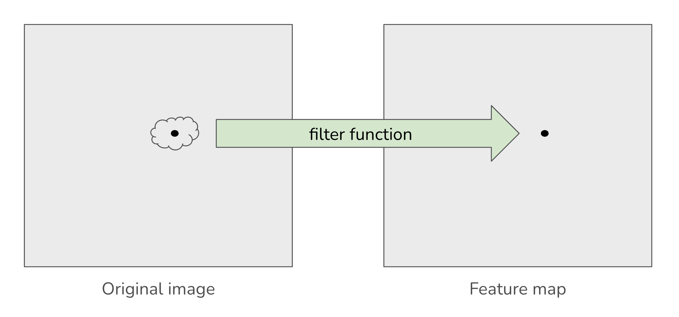
A filter is an image transformation that converts the original image into a new image, usually called a feature map. The value at each location in the feature map is based on the pixel values in a small region surrounding that location in the original image. In other words, a filter looks at the values of pixels in a specified region around some center pixel, and it uses those values to determine the new center value in the feature map.
You can think of this as passing the neighborhood of values through a function that produces a single output value. Figure 1 illustrates this process.
A simple example:
A simple example of a filter is blurring. The blurred image is typically created by averaging the color values of a neighborhood around a pixel. For example, if the neighborhood was defined to be a square 3x3 region, then we would examine every 3x3 region in the image and for each:
- add up all the blue channel values and divide by 9 to get the new blue channel value
- add up all the green channel values and divide by 9 to get the new blue channel value
- add up all the red channel values and divide by 9 to get the new blue channel value
- store the new color at the center location in the new feature map
Blurring is an example of a convolutional filter. These filters have proven to be extremely important in modern deep learning models that operate on images. So we will look more closely at how they work and how they can simplify images and highlight important features in the sections below.
Filtering, generally, can be used to create a number of interesting effects, but is often used to manipulate an image that is then sent to a more complex computer vision algorithm. The main purposes of filtering are:
- Simplifying the image by reducing color variation and/or detail
- Highlighting small-scale patterns in the image, such as edges (places where the brightness changes across neighboring pixels), stripes, color patches, etc.
1.1 What about boundaries!
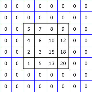
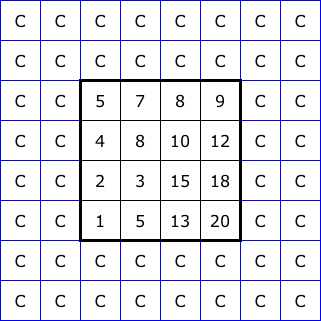
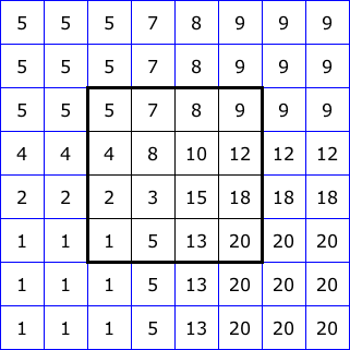
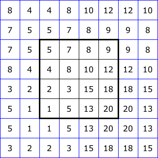
A neighborhood typically is some geometric shape with a center pixel, and the corresponding pixel in the feature map holds the result of the neighborhood calculation. You might wonder what happens to pixels near the boundaries of the image, where they don’t have room for a full neighborhood of pixels around them. The boundary pixels have to be treated as a special case, and wee must define special rules to manage them. Typical rules include:
- Making the feature map smaller than the starting image by leaving out the edge pixels (what Figure 7 below shows)
- Computing the convolution based only on the neighbors that the edge pixels do have
- Imagining that values continue on past the edges of the array and padding the boundary region to create full neighborhoods for edge pixels
Figure 2 illustrates five common ways to “pad” the boundary of an image for filtering. The 4x4 squares at the center of each diagram represent the image itself. Then we show two layers of padding pixels, each assigned values based on a different rule. With this, we could apply a 5x5 neighborhood right up to the edge of the image.
2 Morphological filters
The first filters we will examine are not convolutional in nature. Rather than computing a weighted sum of the values in a neighborhood, morphological filters instead build upon taking the maximum or minimum value in a neighborhood.
All morphological filters operate separately on each color channel (taking the max or min only within the blue channel, or within the green channel, or within the red channel).
The two basic building blocks for morphological filters are dilation and erosion. With dilation, the filter function looks at the values in a neighborhood and keeps the maximum for the corresponding feature map pixel. Erosion is similar, but it keeps the minimum value from the neighborhood.
Below is a list of the morphological filters provided by OpenCV, All of them can be accessed with a single function, morphologyEx, which has many options.
| Operation | Meaning |
|---|---|
| Dilate | Keeps the maximum value from each neighborhood |
| Erode | Keeps the minimum value from each neighborhood |
| Open | First erodes the original, then dilates the result |
| Close | First dilates the original, then erodes the result |
| Top-hat | First opens the original, then subtracts that from the original: Original - Opened |
| Black-hat | First closes the original, then subtracts the original from that: Closed - Original |
| Gradient | Subtracts the eroded image from the dilated one: Dilated - Eroded |
Dilation and erosion are often used to clean up noisy parts of an image, removing dark specks in a light region, for instance, and to even out colors or brightness. They can also thicken or emphasize edges between objects.
Opening and closing are used for similar purposes as dilation and erosion. But they are both more balanced in their effect: because they perform both dilation and erosion, bright and dark regions tend to stay the same size as they were originally.
Top-hat and black-hat are less commonly used, but because they take a difference with either opened or closed images, they keep the fine details that opening and closing are designed to remove. Therefore, they can be used to find textures or to enhance images.
Gradient emphasizes the edges of objects, where dilation and erosion are making the biggest difference.
OpenCV’s morphologyEx function can perform all of these operations. To call it, we pass the image to be filtered a code to tell which operation we want to perform, and a *structuring element, an object that defines the size and shape of the neighborhood.
Unlike most other filters, morphologyEx allows us to have non-rectangular neighborhood shapes. Four default shapes are provided: rectangular, ellipse, diamond, and cross. But you can also define your own shapes if you wish.
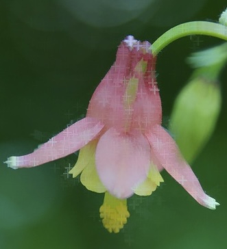
The first code example below loops over the four shapes, and uses them with a dilation operation. Figure 3 shows closeups of the images that result from the same operation, but different neighborhood shapes. It uses a fairly large neighborhood size of 13 by 13 to ensure that the effects are clearly visible.
img = cv2.imread("SampleImages/wildColumbine.jpg")
cv2.imshow("Original", img)

for shape in [cv2.MORPH_RECT, cv2.MORPH_DIAMOND, cv2.MORPH_ELLIPSE, cv2.MORPH_CROSS]:
    structElem = cv2.getStructuringElement(shape, (13, 13))
    newImg = cv2.morphologyEx(img, cv2.MORPH_DILATE, structElem)

    cv2.imshow("Morphed", newImg)
    cv2.waitKey()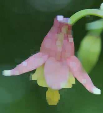
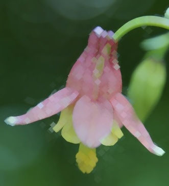
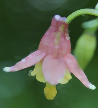
We choose the neighborhood shape depending on the details we want to find in a particular image.
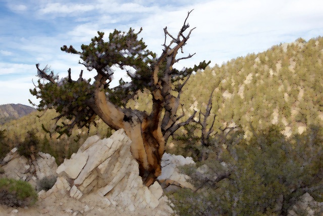
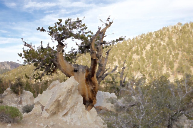
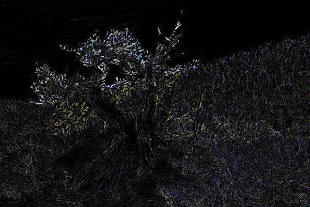
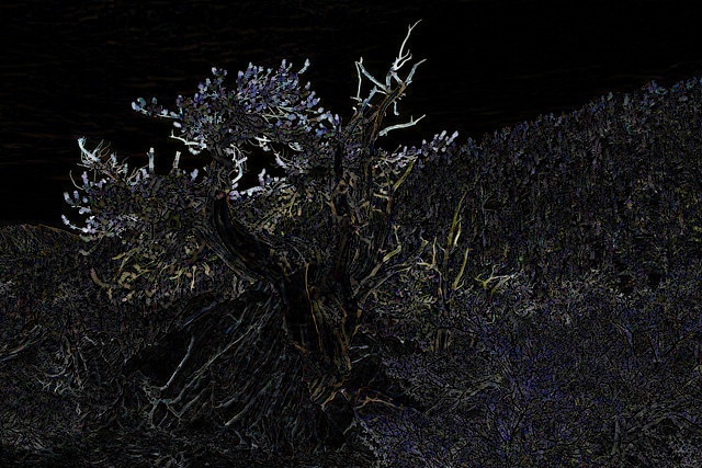
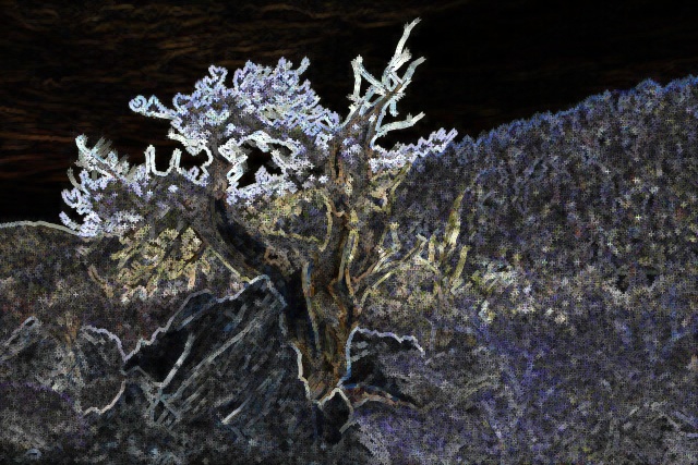
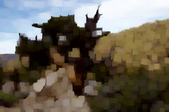
The next example runs each morphological operation on a picture of an ancient bristlecone pine tree. The black-hat and top-hat images use rectangular neighborhoods, the others use the cross shape. Figure 4 shows the original image, and Figure 5 shows the results from the calls in the example below.
img = cv2.imread("SampleImages/bristleconePine.jpg")
cv2.imshow("Original", img)

squareElem = cv2.getStructuringElement(cv2.MORPH_RECT, (5, 5))
crossElem = cv2.getStructuringElement(cv2.MORPH_CROSS, (5, 5))

# Erosion and dilation
erodeIm = cv2.morphologyEx(img, cv2.MORPH_ERODE, crossElem)
dilateIm = cv2.morphologyEx(img, cv2.MORPH_DILATE, crossElem)

# Opening and closing
openIm = cv2.morphologyEx(img, cv2.MORPH_OPEN, crossElem)
closeIm = cv2.morphologyEx(img, cv2.MORPH_CLOSE, crossElem)

# Top-hat and Black-hat
topHatIm = cv2.morphologyEx(img, cv2.MORPH_TOPHAT, squareElem)
blackHatIm = cv2.morphologyEx(img, cv2.MORPH_BLACKHAT, squareElem)

# Gradient
gradientIm = cv2.morphologyEx(img, cv2.MORPH_GRADIENT, crossElem)

cv2.imshow("Erosion", erodeIm)
cv2.imshow("Dilation", dilateIm)
cv2.imshow("Opening", openIm)
cv2.imshow("Closing", closeIm)
cv2.imshow("Top-hat", topHatIm)
cv2.imshow("Black-hat", blackHatIm)
cv2.imshow("Gradient", gradientIm)
cv2.waitKey()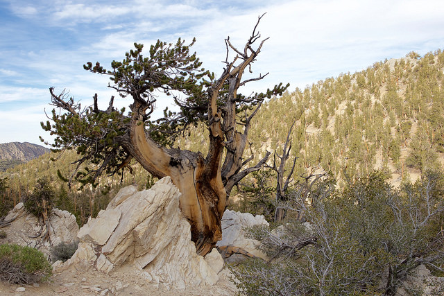
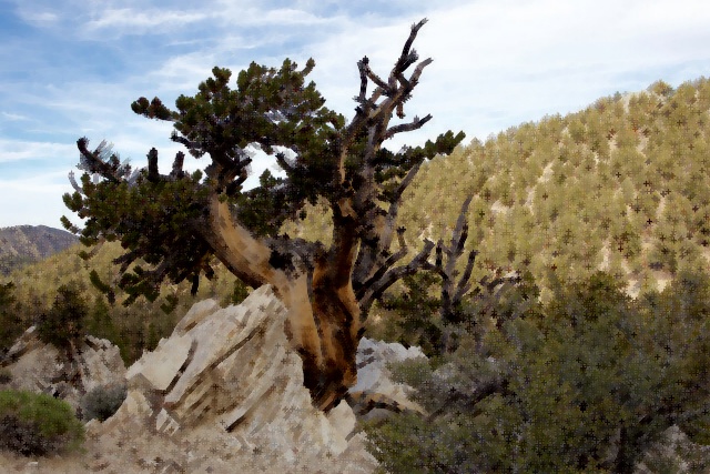
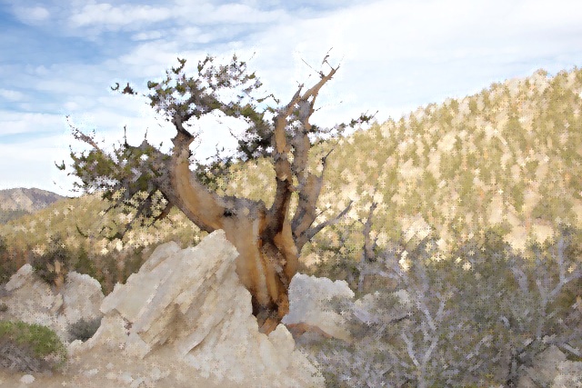
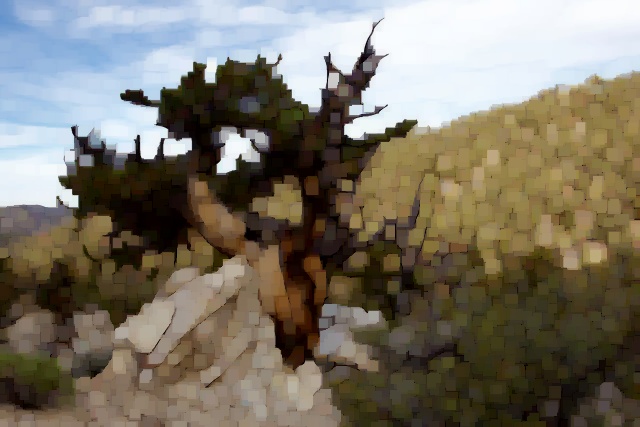
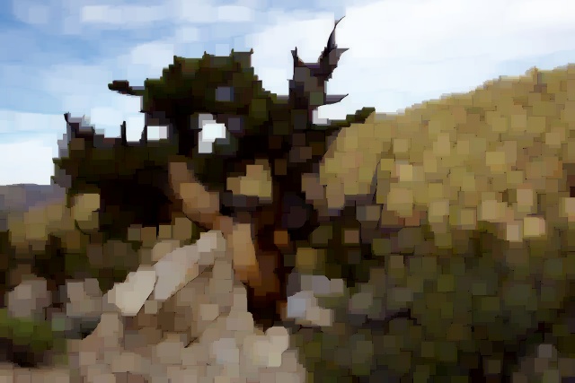
Repeated iterations: There is one last feature of the morphologyEx function to mention to you. As an optional input, you can specify the number of iterations of each operation. If you set iterations to 3, for instance, and then perform an erosion, it will erode the image, then erode the result again, and then erode the result again.
If you perform an operation like opening or closing, that combine erosions and dilations, then increasing the iterations applies to each separate operation. If iterations is set to 2, then opening will first do two erosions in sequence, and then two dilations.
#fig-iterations below shows how increasing the iterations affects the result, given the general form of the code below.
img = cv2.imread("SampleImages/bristleconePine.jpg")
cv2.imshow("Original", img)

morphType = cv2.MORPH_OPEN
morphShape = cv2.MORPH_RECT

for iters in [1, 2, 3, 4]:
    structElem = cv2.getStructuringElement(cv2.MORPH_RECT, (5, 5))
    newImg = cv2.morphologyEx(img, cv2.MORPH_OPEN, structElem, iterations=iters)
    cv2.imshow("Morphed", newImg)
    cv2.waitKey()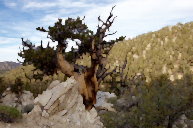
3 Convolutional filters
Convolutional filters are a special kind of filter, where the operation we perform on the neighborhood of pixel values is a weighted sum. We define a kernel: a matrix the size and shape of our neighborhood, where the values in it are weights. For every neighborhood in the image, we multiply pixel values by the corresponding weights in the kernel, and add up the results. The sum is then stored in the corresponding location in the new image/feature map.
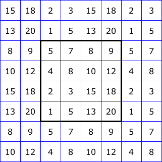
Figure 7 shows the general convolutional process. The grid on the left represents one channel of a tiny image array. The small 3x3 grid in the middle is the kernel of weights. Each weight is multiplied by the corresponding value in the highlighted neighborhood, and the results are added.
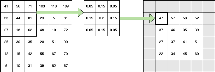
Here is the full sum:
\[ \begin{array}{l} \hspace{5mm} 41 \cdot 0.05 + 56 \cdot 0.15 + 71 \cdot 0.05 \\ + 33 \cdot 0.15 + 44 \cdot 0.2 + 81 \cdot 0.15 \\ + 27 \cdot 0.05 + 18 \cdot 0.15 + 62 \cdot 0.05 \end{array} = 47.05 \]
3.1 A closer look at the math of convolution
Let’s look at the math for a weighted average with a 3x3 neighborhood size.
In convolutional terms, the weights are in the kernel. To simplify the mathematical formula that shows how convolution works, I’m going to label the positions in the kernel in a very non-standard way (I’ll credit OpenCV’s blog on image filtering, and other resources, for using this method to express the convolution formula):
\[ \begin{array}{cc} K & = \begin{bmatrix} K[-1, -1] & K[-1, 0] & K[-1, +1] \\ K[0, -1] & K[0, 0] & K[0, +1] \\ K[+1, -1] & K[+1, 0] & K[+1, +1] \\ \end{bmatrix} \end{array} \]
Generally speaking, we require that the kernel’s dimensions be odd, so an \(n\) by \(m\) kernel can be indexed from \(-\lfloor n / 2 \rfloor\) to \(+\lfloor n / 2 \rfloor\) and from \(-\lfloor m / 2 \rfloor\) to \(+\lfloor m / 2 \rfloor\) putting a single pixel in the middle at (0, 0):
\[ \begin{array}{cc} K & = \begin{bmatrix} K[-\frac{n}{2}, -\frac{m}{2}] & \cdots & K[0, -\frac{m}{2}] & \cdots & K[+\frac{n}{2}, -\frac{m}{2}] \\ \vdots & \vdots & \vdots & \vdots & \vdots\\ K[-\frac{n}{2}, 0] & \cdots & K[0, 0] & \cdots & K[+\frac{n}{2}, 0] \\ \vdots & \vdots & \vdots & \vdots & \vdots\\ K[-\frac{n}{2}, +\frac{m}{2}] & \cdots & K[0, +\frac{m}{2}] & \cdots & K[+\frac{n}{2}, +\frac{m}{2}] \\ \end{bmatrix} \end{array} \]
The convolution formula for an \(n\) by \(m\) neighborhood would look like this:
\[G[x, y] = \sum_{i=-\frac{n}{2}}^{\frac{n}{2}} \sum_{j=-\frac{m}{2}}^{+\frac{m}{2}} K[i, j] \cdot I[x - i, y - j]\]
where \(I\) is the original image, and \(G\) is the resulting image.
4 Blurring filters
Blurring is probably the most basic kind of filter we can do, so we will start by considering it.
Why would we want to blur an image? As humans, we typically don’t like blurred images, unless they are blurred for some effect. However, image data to the computer is just a big box of numbers. Tiny color variations that we are barely aware of can confuse a computer vision program. When we blur an image, those tiny variations smooth out so that colors are more even, and it is easier for a computer vision system to make sense of the image data.
The basic blur function takes a rectangular neighborhood centered around the target pixel, and it performs the mean of the color values, channel-by-channel (all the red values are averaged, all the green values are averaged, and all the blue values are averaged). The resulting color is placed in the new image at the target pixel location. The process is repeated for every pixel in the image (with edge pixels handled specially, as described above)
With blurring we talk about averaging, with convolution we talk about computing a weighted sum. But really, averaging can be thought of as a weighted sum. Below I show formulas for averaging a 3x3 region, then I convert those to the weighted-sum form:
\[ \begin{array}{l} (v_{11} + v_{12} + v_{13} + v_{21} + v_{22} + v_{23} + v_{31} + v_{32} + v_{33}) / 9 \\ \\ \hspace{1cm} = v_{11} / 9 + v_{12} / 9 + v_{13} / 9 + v_{21} / 9 + v_{22} / 9 + v_{23} / 9 + v_{31} / 9 + v_{32} / 9 + v_{33} / 9 \\ \\ \hspace{1cm} = 0.11 v_{11} + 0.11 v_{12} + 0.11 v_{13} + 0.11 v_{21} + 0.11 v_{22} + 0.11 v_{23} + 0.11 v_{31} + 0.11 v_{32} + 0.11 v_{33} \\ \end{array} \]
The kernel for simple blurring has the same value in every cell: \(1/n\), where \(n\) is the number of cells in the neighborhood.
OpenCV provides the blur function, which will perform the simple mean/averaging blur described above. We specify the image to be blurred, and a tuple describing the neighborhood size, it returns a blurred image.
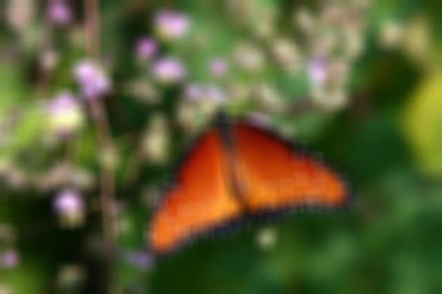
The code block below are some example of how to call the blur function. Figure 8 shows the original and resulting images.
image = cv2.imread("SampleImages/butterfly.jpg")
blur1 = cv2.blur(image, (7, 7))
blur2 = cv2.blur(image, (21, 21))
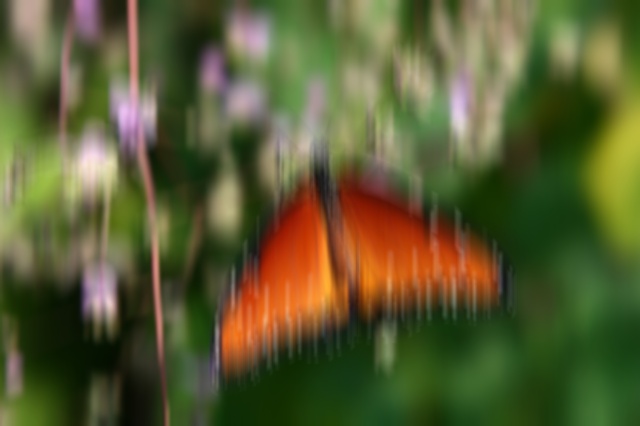
blur3 = cv2.blur(image, (3, 41))
cv2.imshow("Original", image)
cv2.imshow("Blur1 feature map", blur1)
cv2.imshow("Blur2 feature map", blur2)
cv2.imshow("Blur3 feature map", blur3)
cv2.waitKey()

Besides taking a straight average of the color channel values, we can get a blur effect by taking a weighted average of the values in the neighborhood. To do a weighted average with convolution without altering the brightness of the image, we add a constraint that says that the values in the kernel must add up to 1.0:
\[\sum_{i=-\frac{n}{2}}^{\frac{n}{2}} \sum_{j=-\frac{m}{2}}^{+\frac{m}{2}} K[i, j] = 1.0\]
OpenCV provides a weighted blur function called GaussianBlur. This function does a weighted average where the weights are chosen according to a two-dimensional Gaussian function with its peak centered on the center pixel of the neighborhood. Gaussian functions, or curves, are often called normal curves or bell curves. In Chapter 4 we briefly talked about 2d Gaussian curves in the context of the adaptiveThreshold function. Figure 9 illustrates the shape.
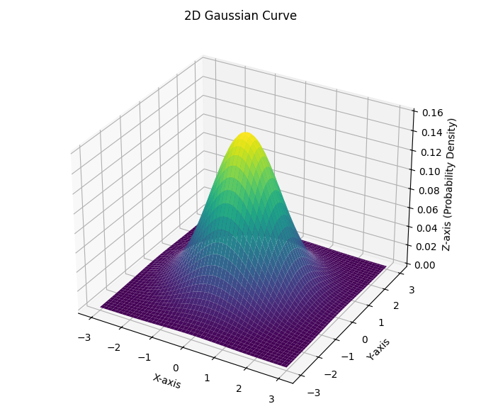
We scale the Gaussian curve to fit our neighborhood size, and so that its values at discrete points add up to one, and those values become our kernel values. Note: Figure 7 uses a kernel that approximates the gaussian blur kernel for a 3x3 neighborhood. The shape of the Gaussian curve is defined by its standard deviation in the x and y directions.
OpenCV provides the GaussianBlur function, which will perform the Gaussian weighted average blur described above. We specify the image to be blurred, a tuple describing the neighborhood size (dimensions must be odd!) and a value for the standard deviation in the x direction. If we pass in zero, then the function determines the best standard deviation values based on the width and height of the neighborhood.
The code block below are some example of how to call the Gaussian function. Figure 10 shows the original and resulting images.
image = cv2.imread("SampleImages/butterfly.jpg")

gblur1 = cv2.GaussianBlur(image, (7, 7), 0)
gblur2 = cv2.GaussianBlur(image, (21, 21), 0)
gblur3 = cv2.GaussianBlur(image, (3, 41), 0)

cv2.imshow("Original", image)
cv2.imshow("GBlur1 feature map", gblur1)
cv2.imshow("GBlur2 feature map", gblur2)
cv2.imshow("GBlur3 feature map", gblur3)
cv2.waitKey()


Why use Gaussian Blur? Compare the results of the Gaussian blur with the simple blur results from earlier in this section. Notice that the Gaussian blur retains more of the detailed features of the image. In practice, Gaussian blurs often do better at simplifying images the way we want, reducing color variations, noise, and tiny zigzags, while preserving more of the features we want to keep, such as edges. There are more elaborate blurring functions as well, including medianFilter and bilateralFilter, but we won’t dig too deeply into those here.
In the SampleCode folder that was provided to you, there is a demo program called blurring.py that you can use to explore these two blurring functions, and the effects of different neighborhood sizes. Run the program, and then use the following keyboard commands to control the effect:
- 1: switches to the simple blur
- 2: switches to the Gaussian blur
- w: increases the height of the neighborhood by 2
- s: decreases the height of the neighborhood by 2
- a: decreases the width of the neighborhood by 2
- d: increases the width of the neighborhood by 2
- q: quits the program
5 Edge Detection
Finding edges and lines in images is one of the classic computer vision tasks. Edges are defined to be locations in an image where the color or brightness changes dramatically. There are different tools for determining these edges; we’ll look at the Sobel gradient operation, and the Canny edge detection algorithm.
Edge detection is usually performed on grayscale images. Thus, we focus on brightness of each pixel. We treat the brightness across the pixels of the image as a three-dimensional surface. The image is thought of as a function of two inputs: \(I(x, y)\) and the value of the function is would be drawn in the third dimension (brighter values are higher on the z axis). When we picture the image this way, edges are places where the image function changes most rapidly from bright to dark (or dark to bright). In other words, edges are the places where the slope of the surface is greatest.
We can use some calculus tools to find where those places are: the derivative of a function gives us the slope, and we just look for the largest and smallest values to see where the edges are.
Fortunately, even if you haven’t studied multivariate calculus, you can still make sense of what these algorithms are doing!
5.1 Sobel Gradient-Finding
Sobel first uses Gaussian blurring on an image to smooth the surfaces in the image, and then it looks for peaks and valleys in the result. In mathematical terms, it computes the first derivative of the function represented by the smoothed image at each pixel location, in either the x direction or the y direction. Thus, the result of Sobel is a floating-point number: large positive or large negative values indicate edges. In order to visualize the results of Sobel, we will have to carefully convert it from floating-point back to 8-bit unsigned integers.
Sobel is an example of a convolutional filter, much like blurring. Its kernel produces floating-point values with a large magnitude when there is a change in brightness. Sobel must be computed in horizontal and vertical directions separately. Below is an example of a 3x3 kernels for Sobel:
Finds vertical edges:
\[\begin{bmatrix} 1 & 0 & -1 \\ 2 & 0 & -2 \\ 1 & 0 & -1 \\ \end{bmatrix} \]
Finds horizontal edges:
\[\begin{bmatrix} 1 & 2 & 1 \\ 0 & 0 & 0 \\ -1 & -2 & -1 \\ \end{bmatrix} \]
Let’s work through a few examples showing how the Sobel kernels work.
Suppose that we have a 3x3 patch of an image with these values in it:
\[\begin{bmatrix} 250 & 100 & 50 \\ 230 & 155 & 20 \\ 200 & 107 & 25 \\ \end{bmatrix} \]
Applying the first Sobel kernel to this, we would get:
\[ \begin{array}{l} 1\cdot 250 + 0\cdot 100 + -1 \cdot 50 + 2\cdot 230 + 0 \cdot 155 + -2 \cdot 20 + 1 \cdot 200 + 0 \cdot 107 + -1 \cdot 25 \\ \hspace{5mm} = 250 + 460 + 200 - 50 - 40 - 25 \\ \hspace{5mm} = 910 - 115 = 795 \\ \end{array} \]
The large positive value tells us that there is a strong edge going from bright to dark left to right (if it was going from dark to bright left to right then the large value would be negative).
Suppose we apply the second Sobel kernel to this example:
\[ \begin{array}{l} 1\cdot 250 + 2\cdot 100 + 1 \cdot 50 + 0\cdot 230 + 0 \cdot 155 + 0 \cdot 20 + -1 \cdot 200 + -2 \cdot 107 + -1 \cdot 25 \\ \hspace{5mm} = 250 + 200 + 50 - 200 - 214 - 25 \\ \hspace{5mm} = 61 \\ \end{array} \]
The small positive values indicates that there is a weak change from top to bottom, but nowhere near as strong as in the other direction.
Finally, suppose we had a patch of our image that looked like this:
\[\begin{bmatrix} 119 & 117 & 118 \\ 116 & 119 & 116 \\ 119 & 118 & 117 \\ \end{bmatrix} \]
Applying the first Sobel kernel to this:
\[ \begin{array}{l} 1\cdot 119 + 0\cdot 117 + -1 \cdot 118 + 2\cdot 116 + 0 \cdot 119 + -2 \cdot 120 + 1 \cdot 119 + 0 \cdot 118 + -1 \cdot 117 \\ \hspace{5mm} = 119 + 232 + 119 - 118 - 232 - 117 \\ \hspace{5mm} = 470 - 467 = 3\\ \end{array} \]
A very small value indicates that there is no meaningful edge here. We would get a similar result with the second Sobel kernel: the result is -1.
When we call Sobel, we tell it which direction to perform the filter (which kernel to use) and what type of data to return. The cv2.CV_32F is a code that the function understand to mean to return the array holding np.float32. The final two numbers tell the function which derivative to take: 1, 0 indicates the derivative in the x direction, and 0, 1 indicates the derivative in the y direction.
- 1
- derivative in x direction: find vertical edges where the change in brightness is from left to right
- 2
- derivative in y direction: find horizontal edges where the change in brightness is from top to bottom
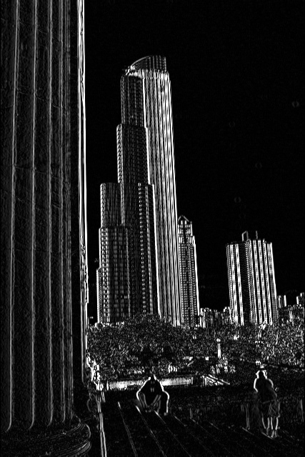
The code example below applies the Sobel filters separately: first to find changes in the x direction, and second to find changes in the y direction. For purposes of precision, the resulting data are 32-bit floating-point numbers. We use the convertScaleAbs OpenCV function to convert negative values to positive, scale them down to 8-bit integers, and then convert them to the correct np.uint8 type.
img = cv2.imread("SampleImages/chicago.jpg")
gray = cv2.cvtColor(img, cv2.COLOR_BGR2GRAY)
# Compute gradient in horizontal direction (detects vertical edges)
sobelValsHorz = cv2.Sobel(gray, cv2.CV_32F, 1, 0)
horzImg = cv2.convertScaleAbs(sobelValsHorz)
cv2.imshow("horizontal gradient", horzImg)
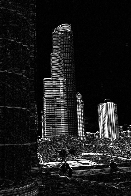
# Compute gradient in vertical direction (Detects horizontal edges)
sobelValsVerts = cv2.Sobel(gray, cv2.CV_32F, 0, 1)
vertImg = cv2.convertScaleAbs(sobelValsVerts)
cv2.imshow("vertical gradient", vertImg)
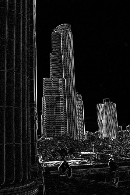
# Combine the two gradients
sobelComb = cv2.addWeighted(sobelValsHorz, 0.5, sobelValsVerts, 0.5, 0)
# Convert combined back to uint8
sobelImg = cv2.convertScaleAbs(sobelComb)
cv2.imshow("Sobel", sobelImg)
cv2.waitKey(0)Figure 11 displays the three results from this sample program. The first detects only vertical edges, and the second only horizontal. But we can blend the two together to get edges in any direction.
5.2 Canny Edge Detection
The Canny algorithm is more elaborate than Sobel: it produces a black and white image where the edges are all one pixel wide. It performs the following steps:
- Apply a gaussian blur to reduce noise in the image
- Perform Sobel in x and y directions, separately
- Perform non-max suppression to reduce edges to one pixel in width
- Perform hysteresis thresholding to keep only strong, connected edges
We’ve already learned about blurring and Sobel.
What is Non-max Suppression? For this, Canny looks at small neighborhoods that are just one row tall, and a few pixels long. If the center point is not the largest in its little neighborhood, then the center point is set to zero. It does the same thing with one-column wide neighborhoods in the vertical direction. This reduces a clump of edge values to just the strongest one.
What is hysteresis thresholding?
This kind of thresholding has two threshold values, the minval and the maxval, passed in when we call Canny. The first threshold should be smaller than the second threshold. Between them, they divide the space of brightness values into three parts: those less than the minval threshold, those in between minval and maxval, and those over maxval. The thresholding works this way:
- Any value under minval is automatically discarded (set to zero)
- Any value over maxval is automatically kept (set to one)
- Values between minval and maxval are only kept if they are adjacent to a pixel that has been set to one. Otherwise, they are discarded
Figure 12 illustrates this process. The curved lines represent edges that have been found in the image, and pixels in the lines are adjacent if drawn that way. The vertical value of each point on the line represents its brightness. And we’ve drawn the minval and maxval thresholds on the figure.
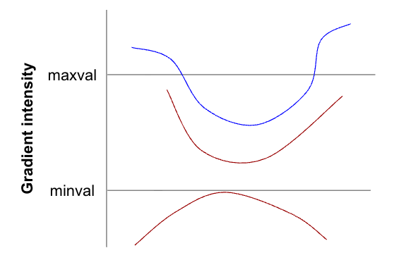
- The bottom line has no pixels above minval. Thus, it is a very weak edge, and all its pixels are discarded and set to zero.
- The middle line lies between minval and maxval. However, at no point does it connect to any pixels that lie above the maxval line, so all of its pixels are discarded
- The top line has ends that are above maxval. Thus initially, those are the only points that would be marked to be kept. However, there are points between minval and maxval that are adjacent to the ones above maxval, so those would be marked to keep, and then their neighbors would be marked, and so on until the entire line is marked to be kept.
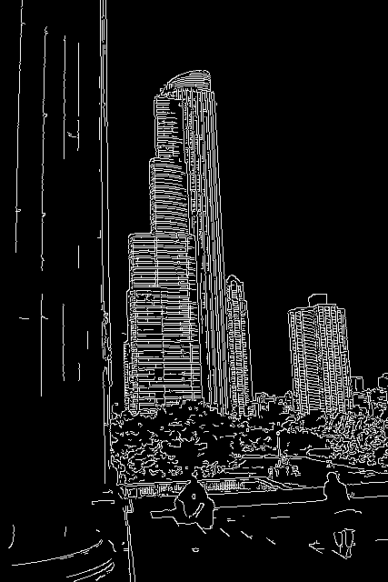
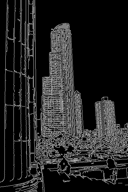
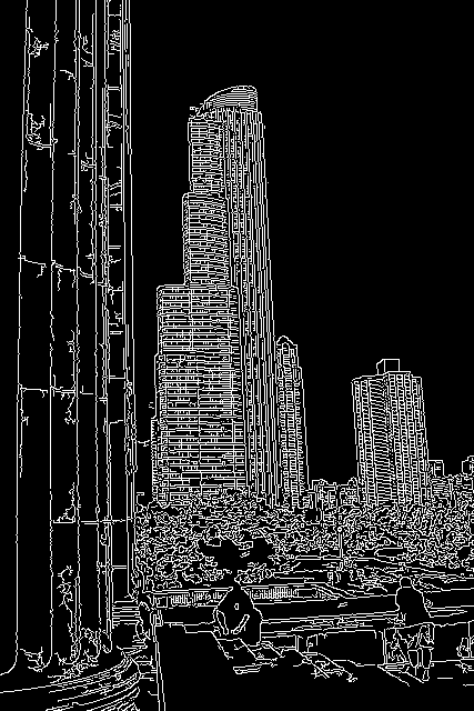
Below is a code example showing the result of running Canny on the same picture as above. Notice that Canny works well when given a color image.
Figure 13 shows the results of this sample program. Notice how changes to each threshold affect the result. Determining the right threshold values can be a matter of art, rather than science (guess at the values and then tweak them until they work for your task). This can make it hard to work with.