In this chapter, we will continue our examination of image transformations with geometric transformations. Geometric transformations are used to resize images, but also to translate, rotate, or warp image contents within the frame of an image.
1 Resizing images
The most basic transformation is resizing an image. The resize function will scale a picture up or down, and can also be used to stretch an image by changing its aspect ratio, the ratio of an image’s width to its height. You must give the resize function a source image and an input for the dimensions of the new image. It has three optional inputs, as well. Two of these let you specify the width and/or height of the new image as a factor of the original, and the last optional input lets you select the interpolation algorithm to be used. Below are some examples of ways to use resize:
| Examples | Meaning |
|---|---|
cv2.resize(src, (100, 100)) |
Returns a new image that is 100 x 100 pixels, a stretched/squashed version of the original |
cv2.resize(src, (0, 0), fx=2, fy=2) |
Returns a new image that is twice the size of the original, same aspect ratio |
cv2.resize(src, (0, 0), fx=0.5, fy=1.0) |
Returns a new image whose columns have been squashed to half the original size |
Interpolation is the process used to make the resized image look better. When we reduce the size of the image, one new pixel might have to cover a part of the image that original had multiple pixels. When we increase the size of the image, we want to smooth the colors where we are adding pixels that weren’t there before, so that the image does not look pixelated. Interpolation determines the colors of the pixels to preserve as much information from the image as possible, while smoothing adjacent pixel values.
According to the OpenCV documentation, The cv2.INTER_AREA interpolation method is best when reducing the size of the image, but cv2.INTER_CUBIC or cv2.INTER_LINEAR (the default method) work best when scaling an image up to a larger size.
Below is a code example that illustrates some changes made to a typical image, followed by the results in Figure 1.

2 Geometric transformations with affine warping
Geometric transformations includes scaling, translation, rotation, reflection, and skewing the contents of an image. The resize function takes care of the scaling part, and the flip function (or just Numpy slicing) can handle reflection. We will use affine warping to perform most of the other kinds of geometric transformations.
- Translation means moving the pixels in an image horizontally and vertically, so the image appears shifted to the right or left, up or down.
- Rotation means moving the pixels so that the image appears to be turned around some specific pixel in the image.
- Skewing, or warping, are more complex transformation. For skewing, imaging taking a rectangular image and transforming it into a parallelogram. For warping, imaging the image is on a flexible surface and we pull, push, stretch or compress the image as a whole into a new shape.
All of these geometric transformations can be thought of in terms of geometry or in terms of linear algebra and matrix operations.
Additional notes:
- A more complex form of geometric transformation is called perspective warping. This treats the image as a part of a plane, and transforms the plane to a new location (as if the image was a printed painting, and we were viewing it moved to a new location).
- For more details about the mathematics underlying geometric transformations, see the blog post on Geeks for Geeks, Geometric Transformation in Image Processing.
Affine warping can be thought of as a set of formulas that map pixel locations in the original image to where that pixel should appear in the new, transformed image. The formulas are shown below:
\[x_{new} = a \cdot x_{old} + b \cdot y_{old} + t_x\]
\[y_{new} = c \cdot x_{old} + d \cdot y_{old} + t_y\]
We can write these in terms of matrix and vector operations, like this:
\[ \begin{bmatrix} x_{new} \\ y_{new} \\ 1 \end{bmatrix} = \begin{bmatrix} a & b & t_x \\ c & d & t_y \\ 0 & 0 & 1 \\ \end{bmatrix} \cdot \begin{bmatrix} x_{old} \\ y_{old} \\ 1 \end{bmatrix} \]
The effect of the transformation depends on the values of the four coefficients, \(a\), \(b\), \(c\), and \(d\), as well as the two constants \(t_x\) and \(t_y\). By varying those six values, we can perform all kinds of geometric transformations. In the next subsections, we’ll take a look at each type of transformation.
2.1 Translation
To translate an image, we want to move every pixel the same distance in the x direction, and the same distance in the y direction. In math terms, this looks like:
\[x_{new} = x_{old} + t_x\] \[y_{new} = y_{old} + t_y\]
Compare this formula to the affine warping formula above, and you can see how we can choose values for \(a\), \(b\), \(c\), and \(d\) to make these formulas out of the original (Let \(a= 1\), \(b = 0\), \(c = 0\), and \(d = 1\)). Because the matrix for translation will always have this simple form, when we program it, we will have to make the matrix ourselves. Look at the 3x3 matrix shown above; since the bottom row is always fixed in value, we only have to specify the top two rows when doing an affine warp in OpenCV.
In the code below, we use the warpAffine function to translate the contents of the image 100 pixels to the right, and 50 pixels down. This function takes in an image, and a 2x3 matrix of floating-point values that specify the six values from the affine warping formulas/matrix. We also tell the function how large to make the output image: it is common to keep it the same size, but we can choose any size we want.
import cv2
import numpy as np
img = cv2.imread("SampleImages/antiqueTractors.jpg")
(hgt, wid, dep) = img.shape
tMatrix = np.matrix([[1, 0, 100], [0, 1, 50]], np.float32)
newIm = cv2.warpAffine(img, tMatrix, (wid, hgt))- 1
- Gets the size of the original, so we can set the new image to that size
- 2
- Makes a 32-bit floating-point matrix with the values for translating in both x and y directions
- 3
- Creates a translated image the same size as the original
Figure 2 shows the result of this transformation.
2.2 Rotation
Rotating an image is closely related to the rotation of axes, a topic you may have studied in school earlier (in the US, it is often covered in precalculus classes). In linear algebra terms, there is a rotation matrix that can perform a rotation. With affine warping, we could build and use a version of this rotation matrix to perform rotations.
However, OpenCV is going to do some of the hard work for us! Instead of us remember the formulas for the affine warping rotation matrix, OpenCV implements a function, getRotationMatrix2d that calculates the correct rotation matrix for us. This function has three inputs: the (x, y) coordinates of the pixel that should be the center of rotation, the angle to rotate by (positive values rotate counter-clockwise), and a scaling factor (in case we want to resize the rotated image at the same time). Figure 3 shows what these inputs mean. We can choose any pixel in the image as the center of rotation. Think of this as a putting a pin at a specific pixel, and then rotating the image around that point. The angle, given in degrees, tells how far to rotate in the counter-clockwise direction.
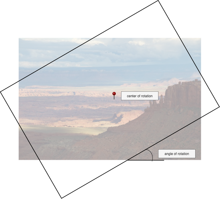
getRotationMatrix2d with center of rotation and angle of rotation specified
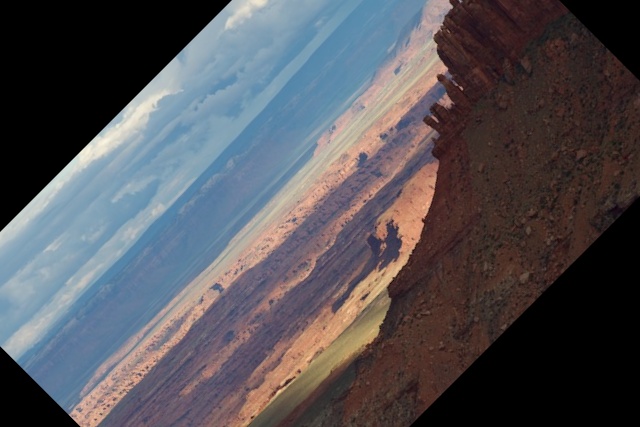
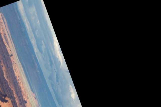
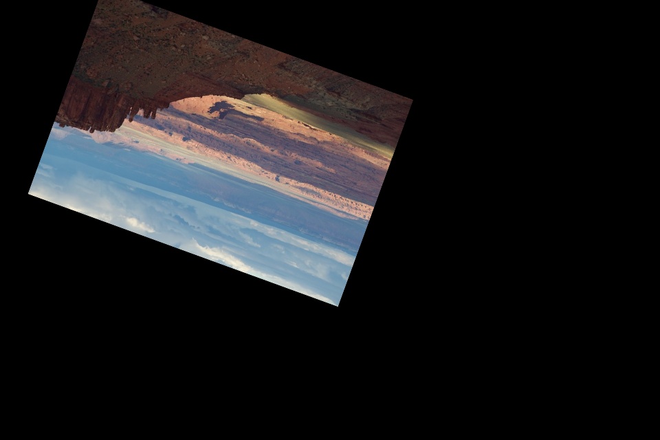
The code example below rotates the image three different amounts, and #fig-rotExamples shows the resulting images.
origIm = cv2.imread("SampleImages/canyonlands.jpg")
(hgt, wid, dep) = origIm.shape

rot1Mat = cv2.getRotationMatrix2D((wid//2, hgt//2), 45, 1)
imRot1 = cv2.warpAffine(origIm, rot1Mat, (wid, hgt))

rot2Mat = cv2.getRotationMatrix2D((100, 100), -70, 1)
imRot2 = cv2.warpAffine(origIm, rot2Mat, (wid, hgt))

rot3Mat = cv2.getRotationMatrix2D((wid//2, hgt//2), 160, 0.75)
imRot3 = cv2.warpAffine(origIm, rot3Mat, (int(1.5*wid), int(1.5*hgt)))
2.3 General affine warping
Besides translation and rotation, the affine warping formulas can be used in ways that skew, twist, and warp the original image. Rather than building the 2x3 matrix by hand, as we did for translation, we will instead use a helper function, like we did for rotation, to build the matrix for us.
The affine warping formulas are fairly simple: just a linear combinations of the old x and old y values. Because of this, we can derive the values for the 2x3 matrix just by knowing how to map a small set of points from the original to locations in the new image. In fact, we only need three points (as long as the points do not all lie in a straight line).
Figure 5 illustrates this process. We pick 3 points, A, B and C, from the original image, and decide where those points should go in the warped image (on the right). Then OpenCV will help us to figure out how to calculate the transformation for all other points. The figure shows four points, rather than three, because the more complex perspective transform requires four points. Affine warping only requires three.
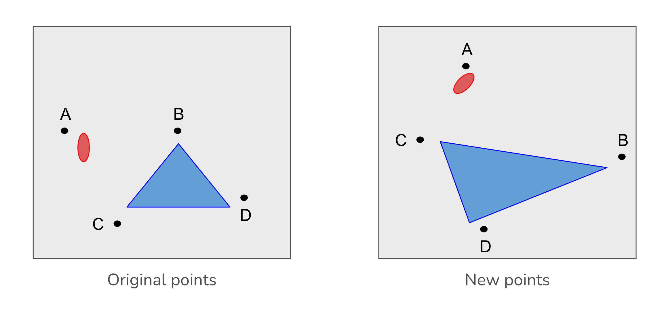
OpenCV provides a helper function, getAffineTransform, that does this derivation. We pass this function two sets of (x, y) coordinates: three points from the original image, and then the points in the new image that should correspond with our three chosen points. In other words, we tell it where we want the three original points to move to in the new, warped image. Specify the points as two Numpy arrays, each with 3 rows and 2 columns, both as 32-bit floating point numbers. Below I show the form of the points arrays, as matrices in math notation.
\[ \begin{array}{cc} origPts = \begin{bmatrix} ox_1 & oy_1 \\ ox_2 & oy_2 \\ ox_3 & oy_3 \\ \end{bmatrix} & newPts = \begin{bmatrix} nx_1 & ny_1 \\ nx_2 & ny_2 \\ nx_3 & ny_3 \\ \end{bmatrix} \end{array} \]
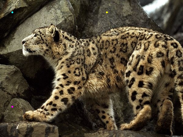
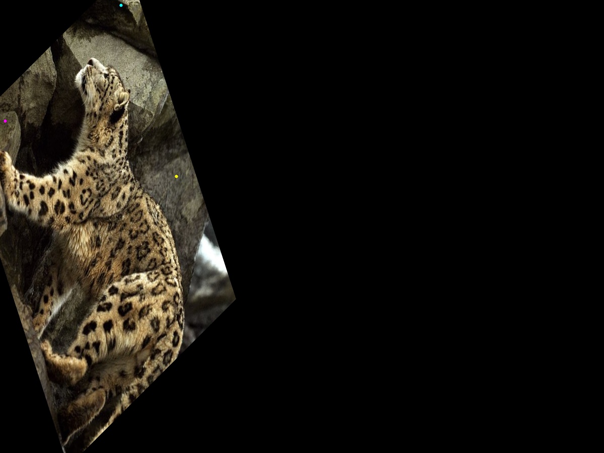
Here is an example of how to create the point matrices, get the affine matrix, and apply it to an image.
import cv2
import numpy as np
img = cv2.imread("SampleImages/snowLeo2.jpg")
cv2.imshow("Original", img)
(rows, cols, depth) = img.shape
origPts = np.float32([[40, 40], [350, 40], [40, 350]])
newPts = np.float32([[240, 10], [350, 350], [10, 240]])
mat = cv2.getAffineTransform(origPts, newPts)
warpImg = cv2.warpAffine(img, mat, (2 * cols, 2 * rows))
cv2.imshow("Warped", warpImg)
cv2.waitKey(0)- 1
-
Creates the array of original points as Numpy’s
float32dtype - 2
-
Creates the array of new points as Numpy’s
float32dtype - 3
- Derive the affine matrix from these two matrices
- 4
- Create the warped image according to the matrix, drawing on a larger image size
In Figure 6 below, we show the original image and the warped one. The warped image is shown on a background image twice as wide and twice as tall as the original. For this, we augmented the code above to draw a small circle at each of the chosen points: cyan for the first pair of points, yellow for the second, and magenta for the third.
2.4 A note about the perspective transform
In addition to affine warping, OpenCV provides another type of warping, the perspective transform. This is based on somewhat more sophisticated, and expensive, math. It simulates the kind of view you would have if the image was printed out on rigid paper, and you looked at it from different perspectives. And it matches the kind of vanishing-point perspective used in art to show realistic depth. When you transform an imate that contains a pair of parallel lines using affine warping, the lines will remain parallel to each other, but they may turn into curved lines. By contrast, if you transform the same image with the perspective transform, the lines will remain straight, but they won’t remain parallel to each other.
Using the perspective transformation is very similar to the affine transformation. You are encouraged to look up the details in the OpenCV documentation.