import cv2
import numpy as np
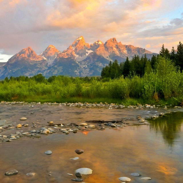
origImg = cv2.imread("SampleImages/grandTeton.jpg")
maskImg = np.zeros(origImg.shape, origImg.dtype) # Makes a copy the same size and type, but all zeros, so black
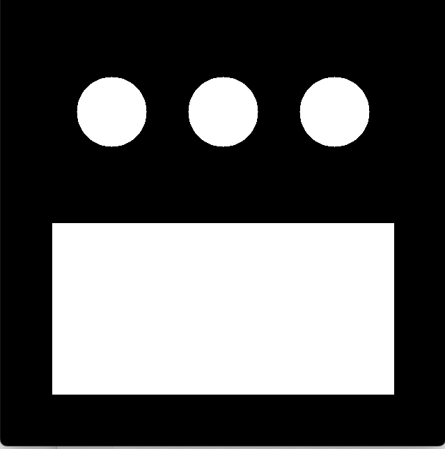
# draw a rectangular region on the mask, and a line of circles
cv2.rectangle(maskImg, (75, 320), (565, 565), (255, 255, 255), -1)
for x in range (160, 640, 160):
cv2.circle(maskImg, (x, 160), 50, (255, 255, 255), -1)
cv2.imshow("Original", origImg)
cv2.imshow("Mask", maskImg)In this chapter, we will examine several approaches for transforming images: taking in an image, and producing a new, changed image. First we will examine the process of masking an image, using a black-and-white image to determine which pixels to keep in an image. And then we will look at several methods for building threshold images, which are typically grayscale or black-and-white, and which separate pixels with certain properties from pixels that lack those properties.
1 Masking images
When we mask an image, we cover over portions of the image, allowing only selected portions to be visible. To mask an image, we must first create a mask image: a special image that has only black and white pixels. The black portions of the mask image are where we will cover up the original image, and the white portions are where we will let the original image show through.
One way to picture this process, is to imagine we have a printed photograph of some kind. If we take a black sheet of paper, and cut holes in it, and then lay it over the printed photograph, that is what masking does. The white parts of the mask image are the holes in the black paper.
There are multiple ways of creating masks. The most simple is to just make a black image and then draw on it the regions we can to keep in the original image. The code example below does exactly this, using OpenCV’s drawing functions to create a black and white mask image.
Figure 1 shows the original image and the mask image constructed by the code.
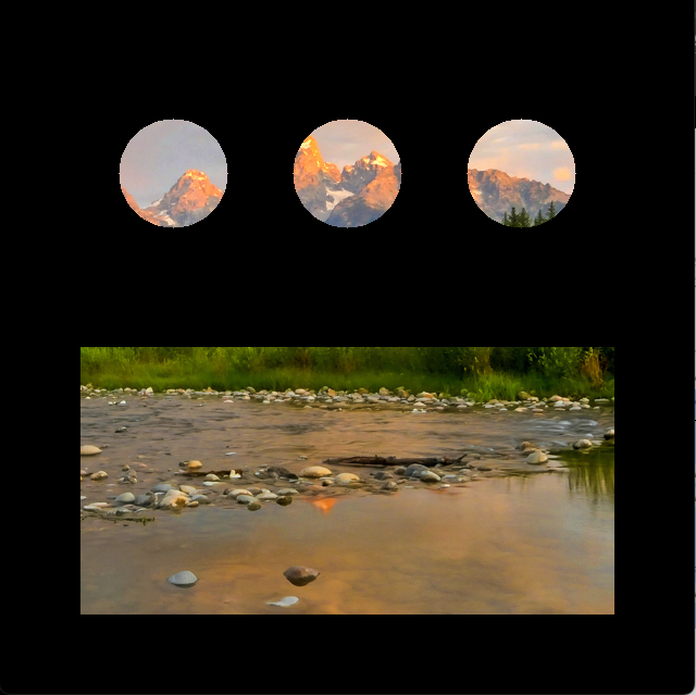
To apply the mask to the original image, we will use the OpenCV function bitwise_and. This is an arithmetic function on images. It takes two images the same size and shape, and it combines them using the bitwise and operation. You don’t need to know all the details, just this: bitwise-and of a color and white returns the color, bitwise-and of a color and black returns black. This gives us the effect we want: the original colors where the mask was white, and black where the mask was black. Below is a continuation of the script above showing how to apply the mask, and Figure 2 shows the result of this operation.
1.1 Three-channel versus one-channel masks
The mask image above was created as a color image, with three channels. If the only colors in a mask are white or black, we don’t really need all three channels. However, when we have a one-channel mask, applying it to the image is a little bit different.
The script below demonstrates several ideas:
- How to apply a mask to frames of a video feed
- How to apply a one-channel mask to a color image
- How to make a square bounce around a window
We’ll discuss each of these ideas as they appear in the code below. Be sure to read the annotations on the lines of code before continuing.
vidCap = cv2.VideoCapture(0)
sqrX = 50
sqrY = 50
deltaX = 5
deltaY = 5
sqSize = 400
while True:
res, frame = vidCap.read()
(hgt, wid, dep)= frame.shape
# make mask a grayscale image (one channel)
maskIm = np.zeros((hgt, wid), np.uint8)
cv2.rectangle(maskIm, (sqrX, sqrY), (sqrX + sqSize, sqrY + sqSize), 255, -1)
maskedFrame = cv2.bitwise_and(frame, frame, mask=maskIm)
cv2.imshow("Moving Mask", maskedFrame)
x = cv2.waitKey(10)
if x > 0:
if chr(x) == 'q':
break
if (sqrX + sqSize >= wid) or (sqrX <= 0):
deltaX = -deltaX
if (sqrY + sqSize >= hgt) or (sqrY <= 0):
deltaY = -deltaY
sqrX += deltaX
sqrY += deltaY
vidCap.release()- 1
- Sets up variables to hold the size and position of the mask square, and how fast it will change from one frame to the other
- 2
-
Gets the shape of the frame into
hgtandwidvariables, so we can make a one-channel mask - 3
- Creates the mask and draws a white square on it
- 4
-
Applies the mask to the frame from the camera feed (or video file), using the
maskinput - 5
- Displays the result
- 6
-
Changes
deltaXand/ordeltaYif the square gets to any of the four edges of the picture; causes the square to change the direction it moves - 7
-
Updates the position of the square for the next frame, by adding
deltaXtosqrXanddeltaYtosqrY
The first part of the while loop creates the mask with one white square, and applies it to the original image. To understand how one-channel masks can be applied to an image, focus on line 17. We cannot just call bitwise_and and pass it the original frame and the mask, because bitwise_and requires that the two images passed to it are the same shape. However, bitwise_and takes an optional input called mask, which specifies a one-channel mask, which is applied to the result of the bitwise-and operation. So we pass the original frame in for both ordinary inputs (bitwise-and applied to two identical images produces the image itself again). And then the mask gets applied in a separate step. This is cryptic and weird, but it works!
The last idea in this code, making a shape bounce around a window, is just for fun, and to emphasize that for each frame in the video feed, we compute and apply a new mask. The key to moving the square is just to change the position of its upper left (x, y) coordinates, which is done at the end of the while loop. To keep the square from just moving out of view, we need to make it bounce back. This sounds daunting, but is actually easy.
- If the right edge of the square reaches or exceeds the right edge of the image, then we change the
deltaXvalue to be its negative (it will have been +5, after this it will be -5) - If the left edge of the square reaches or exceeds the left edge of the image, then we change
deltaXto be its negative (it will have been -5, –5 = +5) - Similar logic for the top and bottom edges
Try this code for yourself. To fully understand this code, you should experiment with changing the accumulator variables (one at a time) that control the position, size, and movement speed of the square. Or change the rectangle to a circle or an ellipse.
1.2 Masks built from image features
Besides building masks as we have done here, by drawing white shapes on a black image, we can also generate mask images using other image transformations, so that the pixels that are white fit some pattern or criteria. Later in this chapter, we will look at a common way to create these masks: computing threshold images.
2 Converting images from ‘BGR’ to other color representations
Some of our image manipulations will require us to change from the normal BGR representation of an image to other forms, including grayscale and HSV. OpenCV gives us one function that can convert between all the implemented color representations: cvtColor. This function takes in an image and a code that tells it which conversion we want, and it returns the converted image. The script below shows how to convert an image to grayscale and to HSV.
Figure 3 shows the original image next to the grayscale version. The imshow function recognizes grayscale images, which have only one channel, and can display them correctly.
A warning about HSV: HSV images have three channels and use np.uint8 as the data type, just like BGR ones. To the computer, these image representations look identical! A function that expects a BGR image and is given an HSV one will interpret the hue channel as a blue channel, the saturation channel as a green one, and the value channel as red. The imshow function assumes that an image with three channels is BGR, so if we try to display an HSV image, we get an odd result, as shown in Figure 4
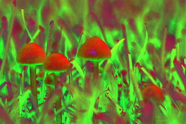
imshow
3 Thresholds from grayscale images
Threshold functions transform images based on the range of grayscale brightness or color values at each pixel. They often produce a black and white image. Threshold images are suitable for use as a mask, but we can also use the threshold image to locate interesting objects in the image.
3.1 The threshold function
The simplest threshold function is called just threshold. It operates on grayscale images, and has multiple modes to choose from. It returns a new grayscale or black and white image.
The threshold function takes in four inputs and returns two results. The four inputs include: a source image, a threshold value (between 0 and 255), a maximum value (also between 0 and 255), and a constant that defines which threshold variant to perform. Table 1 shows the five main variants for this function.
| Threshold mode | Meaning |
|---|---|
cv2.THRESH_BINARY |
Values above the threshold are set to the maximum value, values less than or equal to the threshold are set to zero |
cv2.THRESH_BINARY_INV |
Values above the threshold are set to zero, values less than or equal to the threshold are set to the maximum value |
cv2.THRESH_TRUNC |
Values above the threshold are set to the threshold value, values less than or equal to the threshold are unchanged |
cv2.THRESH_TOZERO |
Values above the threshold are left unchanged, values less than or equal to the threshold are set to zero |
cv2.THRESH_TOZERO_INV |
Values above the threshold are set to zero, values less than or equal to the threshold are left unchanged |
The threshold function returns two values. The first returned value is the threshold value. This may seem odd, but the function has optional add-ons that use particular algorithms to guess at the most useful threshold value. In those cases, we do want the function to tell us the value the algorithm chose. The second returned value is the threshold image itself.
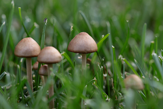
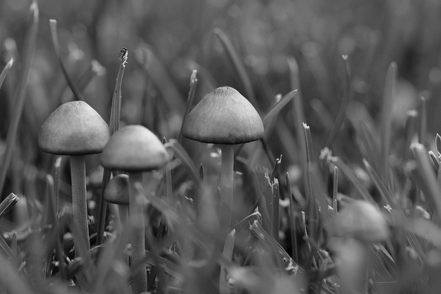
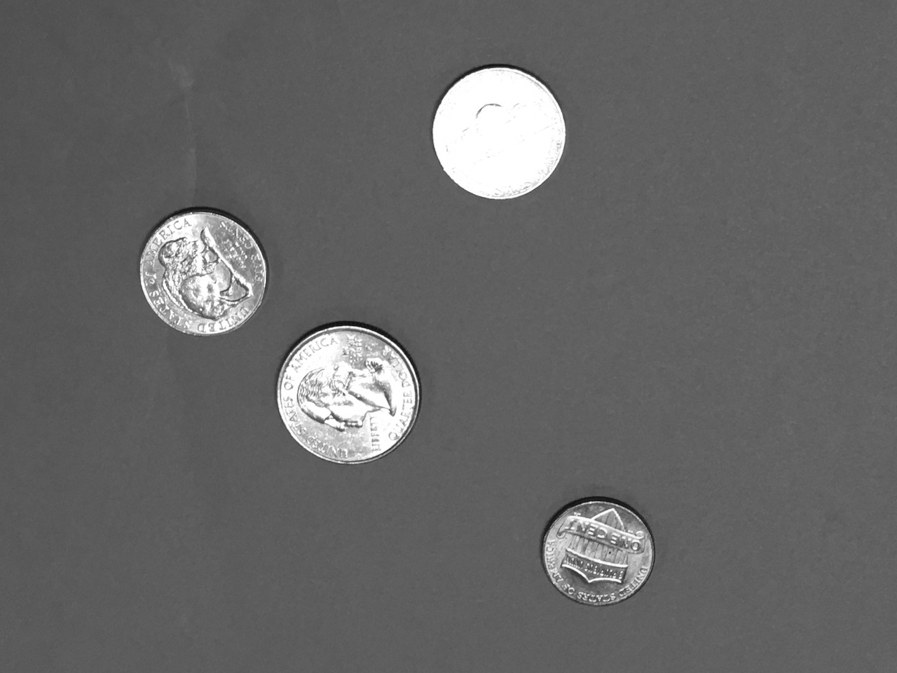
The script below illustrates the threshold function, in all its main variants, on a picture of coins on a red background (found in the Coins folder inside SampleImages). Figure 5 shows the original image, its grayscale counterpart, and then all the five variants.
coinImg = cv2.imread("SampleImages/Coins/coins6.jpg")
grayCoin = cv2.cvtColor(coinImg, cv2.COLOR_BGR2GRAY)

cv2.imshow("Original", coinImg)
cv2.imshow("Gray", grayCoin)
cv2.waitKey()

threshModes = [cv2.THRESH_BINARY, cv2.THRESH_BINARY_INV, cv2.THRESH_TRUNC, cv2.THRESH_TOZERO, cv2.THRESH_TOZERO_INV]
for threshMode in threshModes:
    res, threshIm = cv2.threshold(grayCoin, 128, 255, threshMode)
    cv2.imshow("Threshed", threshIm)
    cv2.waitKey()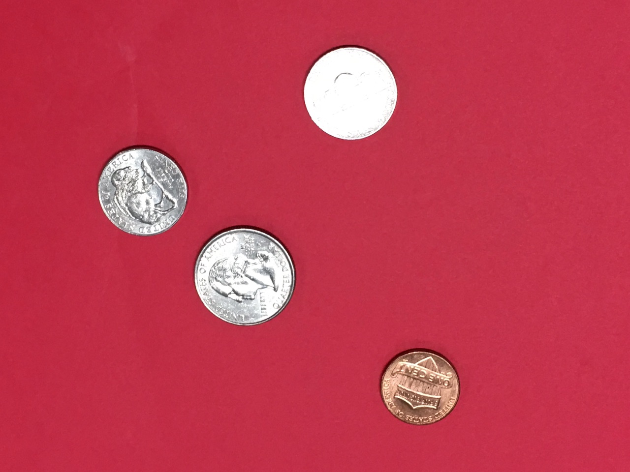

THRESH_BINARY mode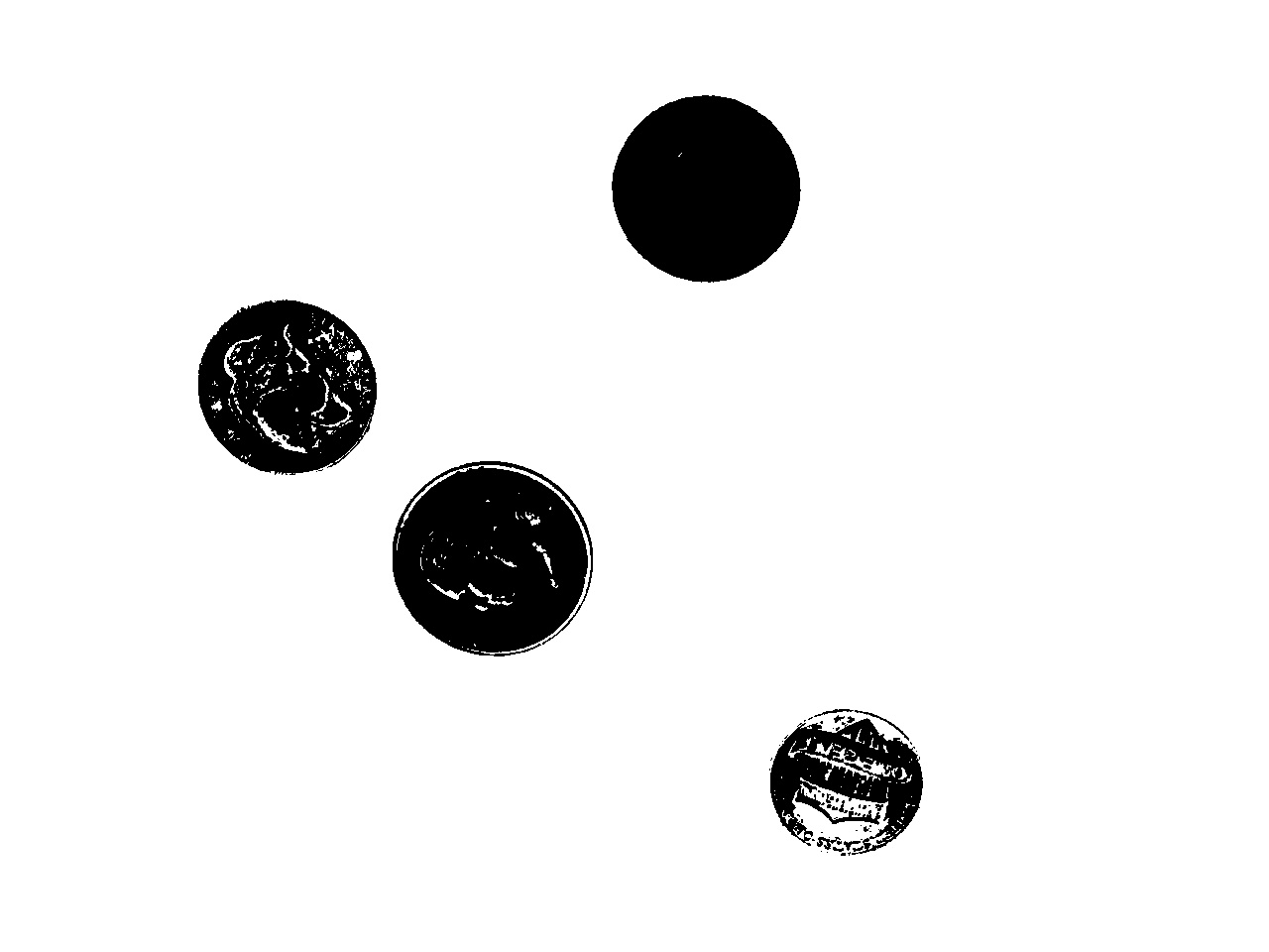
THRESH_BINARY_INV mode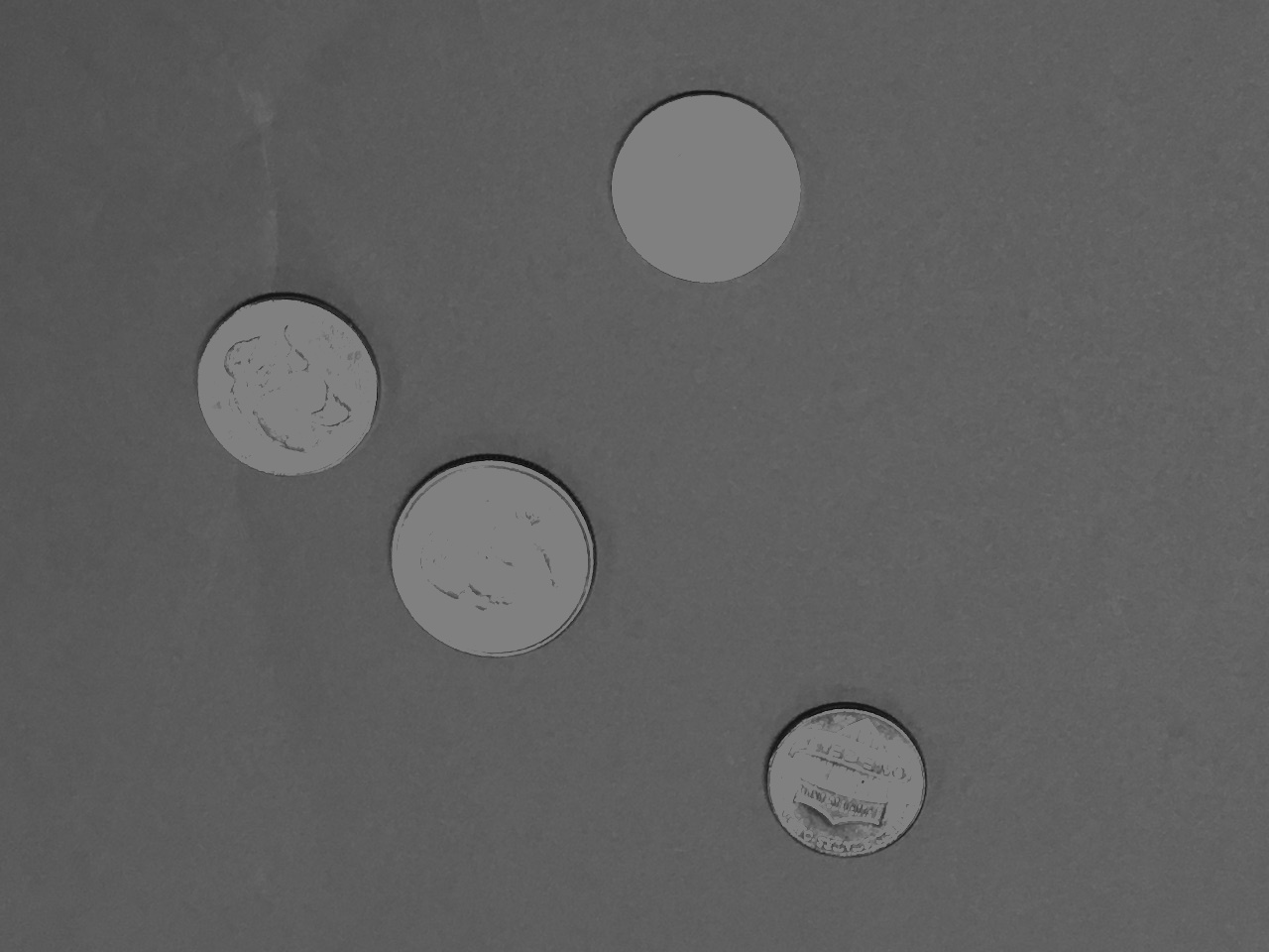
THRESH_TRUNC mode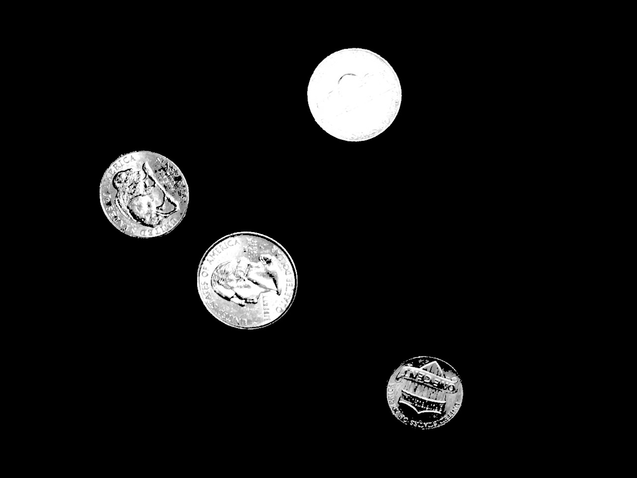
THRESH_TOZERO mode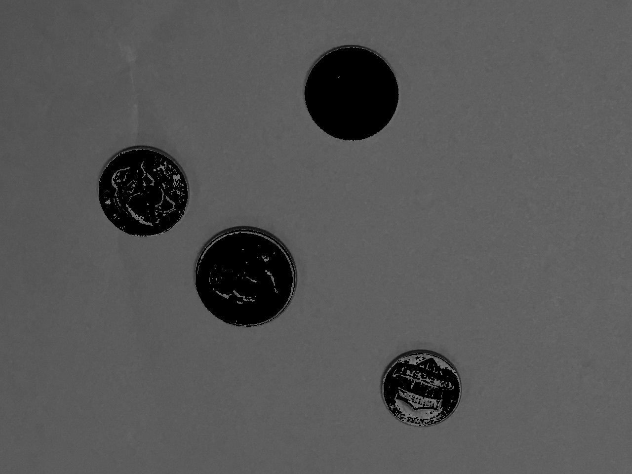
THRESH_TOZERO_INV modethreshold function, all run with threshold value of 128 and max value of 255
One issue with thresholdis determining what the best threshold value is. Algorithms exist that can identify good threshold values for you, and two of them are integrated into the threshold function. The OTSU and Triangle algorithms both build a histogram of the brightness values in a grayscale image. The OTSU algorithm looks for a threshold value that minimizes the variance on each side of the threshold in the histogram. The Triangle algorithm draws a line between the maximum histogram and the minimum one, and finds the point along that line that is maximal distance from values in the histogram, and uses that as the threshold value. (For more information about both algorithms, see OTSU’s Wikipedia page, or David Landup’s blog on StackAbuse.com).
Below is a variation on the code above that shows how to use OTSU or Triangle, combining it with the binary threshold mode. Figure 6 illustrates the results on the coins pictures of each of these algorithms. Note that when we use these algorithms, threshold ignores the input threshold value, and computes its own. It then returns the computed threshold value as its return value.
coinImg = cv2.imread("SampleImages/Coins/coins6.jpg")
grayCoin = cv2.cvtColor(coinImg, cv2.COLOR_BGR2GRAY)

# Adaptive threshold with OTSU and Triangle algorithms
adaptMode1 = cv2.THRESH_BINARY + cv2.THRESH_OTSU
adaptMode2 = cv2.THRESH_BINARY + cv2.THRESH_TRIANGLE
for tm in [adaptMode1, adaptMode2]:
    res, threshIm = cv2.threshold(grayCoin, 128, 255, tm)
    print(res)
    cv2.imshow("Threshed", threshIm)
    cv2.waitKey()
THRESH_BINARY + THRESH_OTSU mode, chose threshold value of 161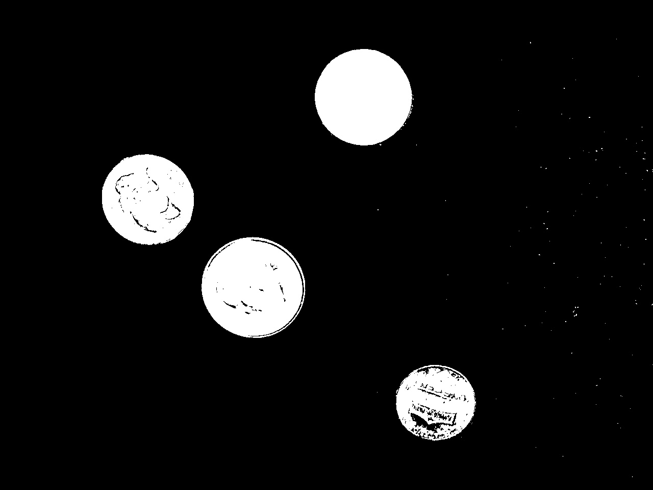
THRESH_BINARY + THRESH_TRIANBLE mode, chose threshold value of 105threshold function, usually added to the binary or to-zero threshold modes.
Think about this: Of all of these approaches, which work best on this picture? Experiment with this code, trying it on the other coin pictures in SampleImages. Does the same version or the same threshold, work for all pictures?
3.2 Adaptive threshold
The adaptiveThreshold function takes things a step further. Rather than just determining one global threshold value, it throws out the idea of a global threshold value altogether. Instead, it computes an individual threshold value at each small patch in the image (this is really a form of filtering, which is the next main subject in the next chapter!).
The function does the same operation on every overlapping patch in the image. It computes either a plain average or a weighted average of the brightness values in the patch, and subtracts a constant c that we provide. This value is the threshold value for the center pixel of the patch. thus different parts of the image may have very different threshold values.
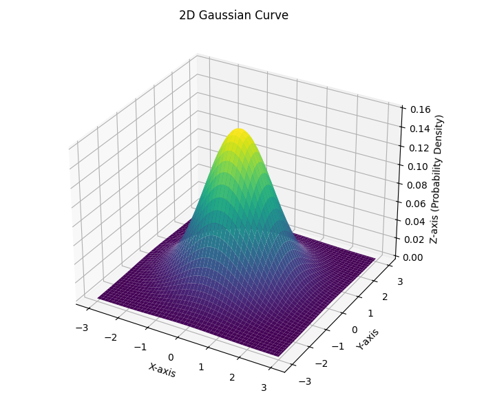
An input constant selects whether to do a plain average or a Gaussian one. We typically describe an ordinary average as adding up the values in the patch and dividing by the number of values. But we can also think of it as multiplying every value in the patch by one over the number of values (if there are \(n\) pixels in a patch, by \(1/n\), and then adding up the results. A Gaussian average is also computed by multiplying every value in the patch by a weight value and then adding the results. However, instead of using the same weight at every position, we choose weights so that they (1) add up to 1.0, and (2) form a Gaussian curve (also called a Normal curve, or a bell curve.). Figure 7 depicts a typical two-dimensional Gaussian curve. This weights values at the middle of the patch highest, and those at the edge of the patch lowest, in a systematic way.
The adaptiveThreshold function takes six (6!) inputs, outlined below:
- The grayscale image to be processed
- The maximum value for the thresholding mode
- The adaptive effect, one of
cv2.ADAPTIVE_THRESH_MEAN_Corcv2.ADAPTIVE_THRESH_GAUSSIAN_C(see discussion above) - The threshold mode, same ones as the
thresholdfunction takes - The size in pixels of the patch to use (use an odd number so that there is always a center pixel)
- The value of
c, a constant that will be subtracted from the average that is computed to produce the threshold value
The code example below loops over different values for the patch size (called bSize because patches are called blocks), and different values for the c constant. We often have to experiment to find the right combination of these values to get the result we want.
for bSize in [3, 5, 7, 11]:
    for c in [2, 5, 10, 20]:
        adaIm1 = cv2.adaptiveThreshold(grayCoin,
                                       255,
                                       cv2.ADAPTIVE_THRESH_MEAN_C,
                                       cv2.THRESH_BINARY,
                                       bSize,
                                       c)
        adaIm2 = cv2.adaptiveThreshold(grayCoin,
                                       255,
                                       cv2.ADAPTIVE_THRESH_GAUSSIAN_C,
                                       cv2.THRESH_BINARY,
                                       bSize,
                                       c)
        print(bSize, c)
        cv2.imshow("Adaptive Mean_C", adaIm1)
        cv2.imshow("Adaptive Gauss_C", adaIm2)
        cv2.waitKey()
Notice how the calls to adaptiveThreshold are formatted, with one input per line. This is a common Python style: if the arguments to a function run too far to the right, rather than just breaking them up wherever, we put one per line, and line them up under the start of the first input.
Figure 8 shows pairs of values, one for the mean, and one for the Gaussian average, for different values of bSize and c.

Mean, bSize = 3, c = 2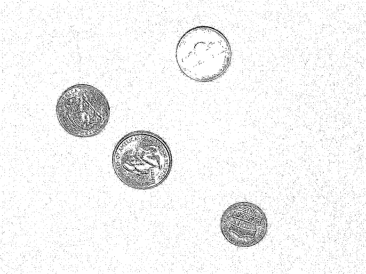
Gauss, bSize = 3, c = 2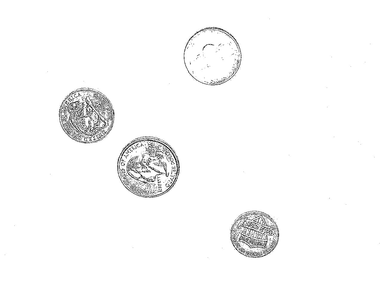
Mean, bSize = 3, c = 5
Gauss, bSize = 3, c = 5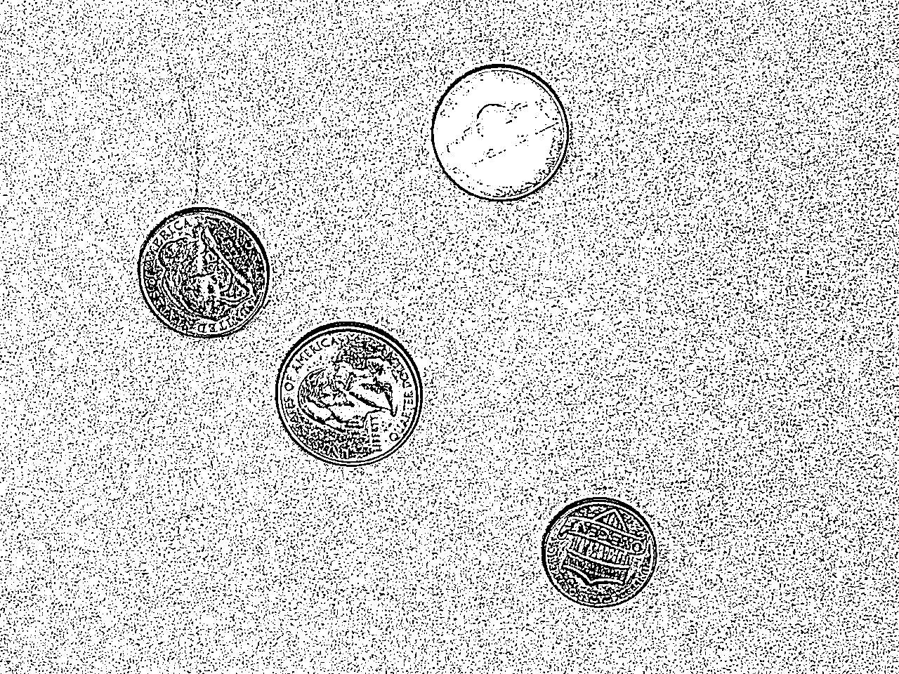
Mean, bSize = 7, c == 2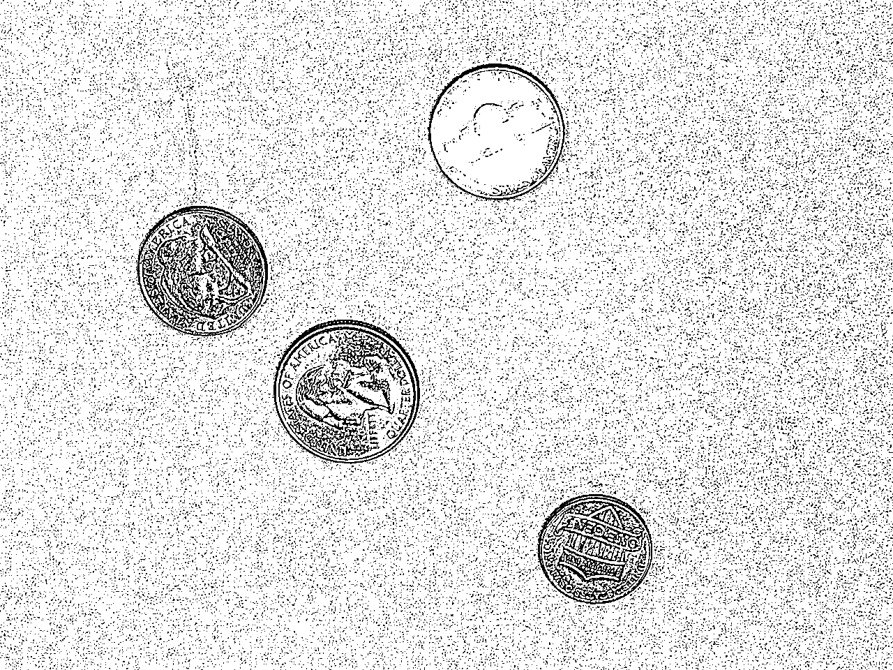
Gauss, bSize = 7, c = 2
Mean, bSize = 7, c = 5
Gauss, bSize = 7, c = 5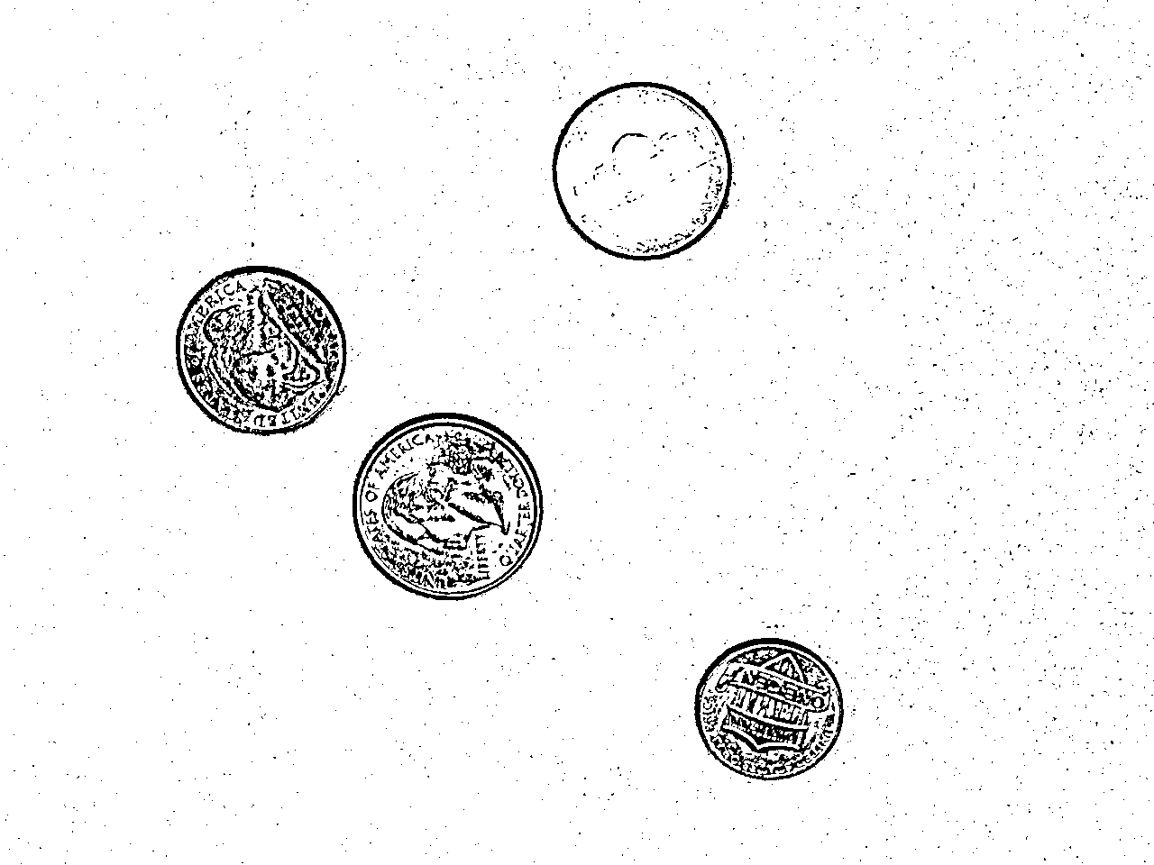
Mean, bSize = 11, c = 5
Gauss, bSize = 11, c = 5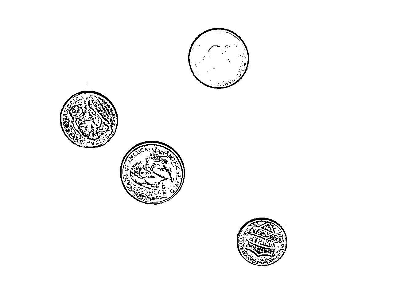
Mean, bSize = 11, c = 10
Gauss, bSize = 11, c = 10adaptiveThreshold given different averaging and values of bSize and x
4 Thresholds from color images
Grayscale as a basis for finding objects in images is limited. We could have a red ball on a green background where they happen to have similar brightness levels. We often want to detect objects by their colors, so there is a threshold function that does just that: inRange. This function takes in a color image, plus two tuples that specify low and high values for each channel, and it returns a threshold image. The returned image is white for pixels where all channel vaues fall within the range we’ve given for that channel.
We can use inRange on BGR images, but BGR color values change in complex ways when the lighting varies: all three channels must increase to produce a brighter version of a given hue, for instance. Instead we will typically convert the image to HSV and then use inRange. If we want to detect a certain color, we can use a narrow range of hue values, but let the saturation and value cover most of the range.
OpenCV adaptation of HSV: If you look at a color wheel to explore HSV values for colors, you will notice that the hue channel typically ranges from 0 to 359 (degrees around a circl), while the saturation and value channels often range either between 0.0 and 1.0 or betwen 0 and 100. OpenCV wants to use 8-bit unsigned integers to represent HSV channels; those are restricted to 0 to 255. The typical range of hue values will not fit in an 8-bit unsigned integer, and the typical range of saturation and value would use less than half of the range available. Thus, OpenCV implements a variation on the typical HSV representation:
- OpenCV uses the range from 0 to 180 to represent hues (take the typical hue and divide by 2)
- OpenCV maps saturation and value numbers on to the full range from 0 to 255
Below is a script that detects a green ball in an image using inRange. It also shows what happens if we try to isolate the ball in the image using threshold, even with the threshold adaptation OTSU in use. Color images just hold more information than grayscale ones.
ballImg = cv2.imread("BallFinding/Green/Green1BG1Mid.jpg")
grayBall = cv2.cvtColor(ballImg, cv2.COLOR_BGR2GRAY)
hsvBall = cv2.cvtColor(ballImg, cv2.COLOR_BGR2HSV)
threshImg1 = cv2.inRange(hsvBall, (45, 10, 0), (65, 255, 255))
res, threshImg2 = cv2.threshold(grayBall, 128,255, cv2.THRESH_BINARY+cv2.THRESH_OTSU)

cv2.imshow("inRange", threshImg1)
cv2.imshow("threshold", threshImg2)
cv2.waitKey()
Figure 9 shows the original image, the grayscale version, and then the results of the calls to inRange and threshold.
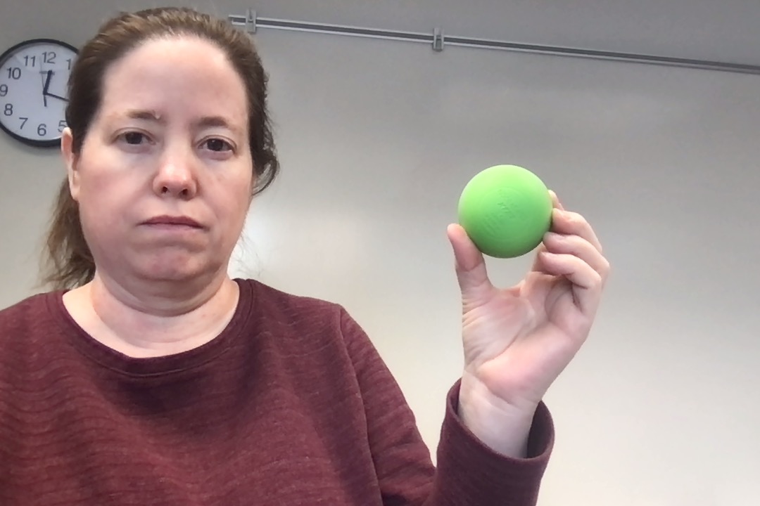
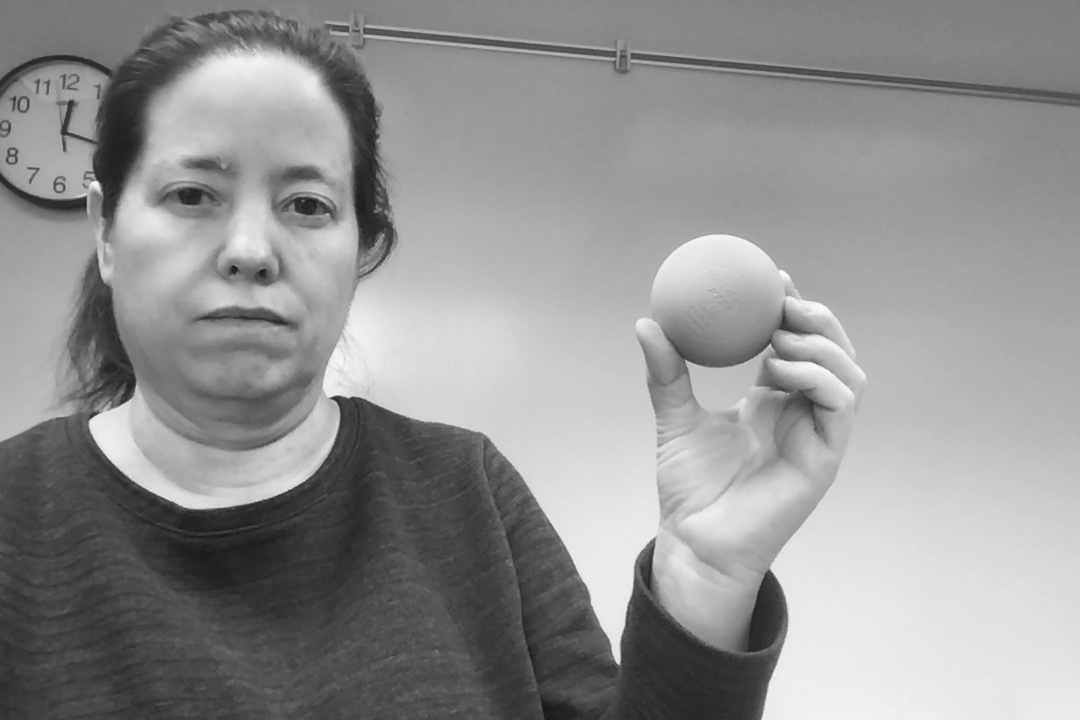
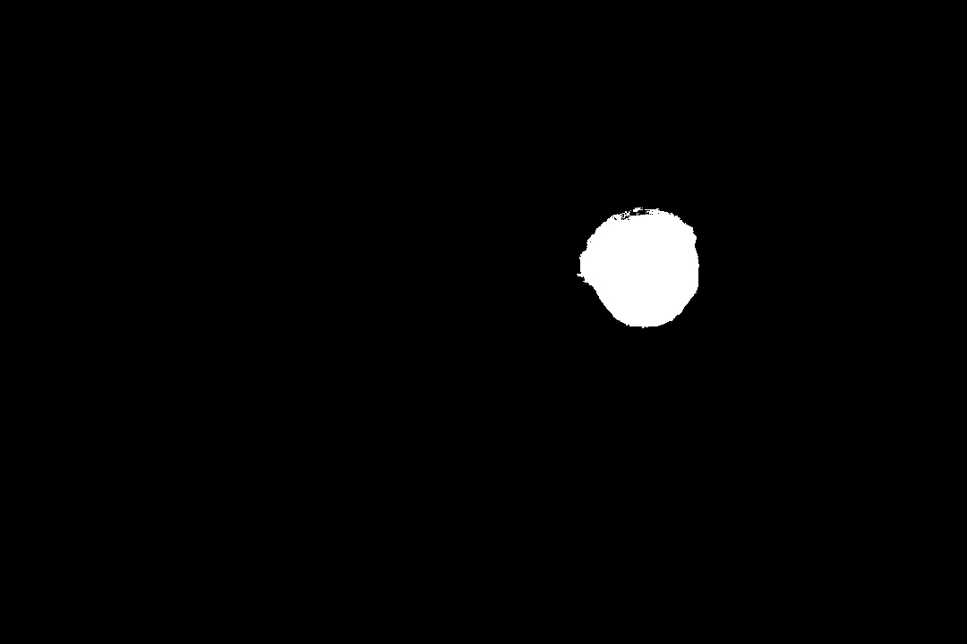
inRange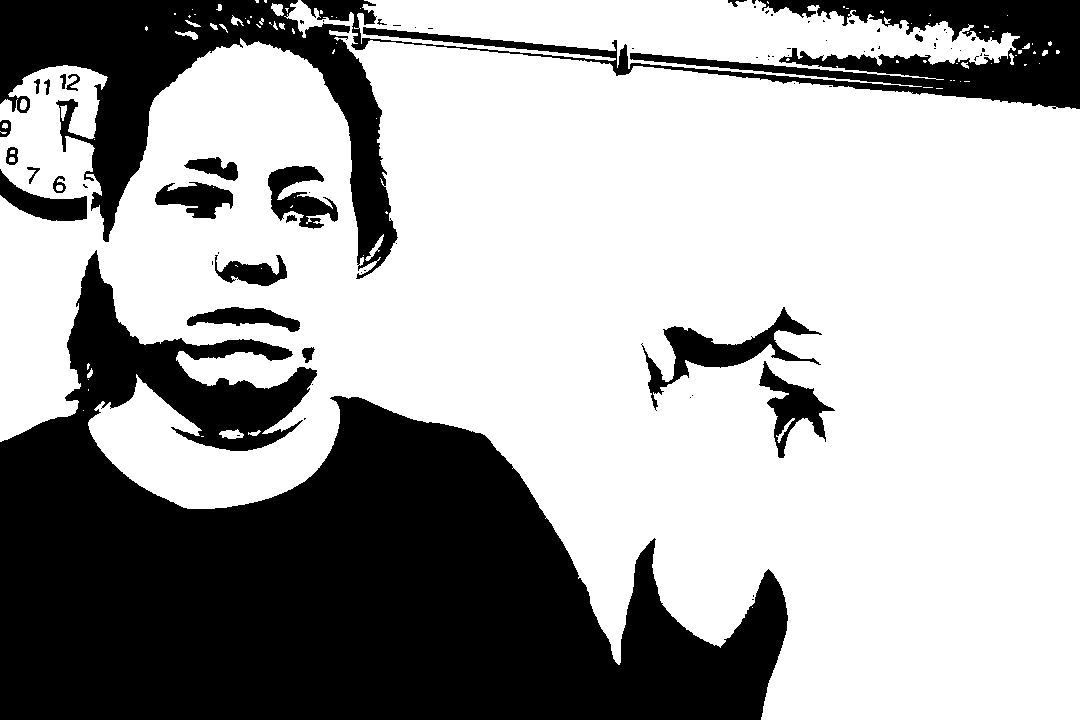
threshold with OTSUinRange and theshold on an image, seeking to isolate the green ball from the rest of the image
We encourage you to try this on some of the different colors of balls in the BallFinding folder. There are two main drawbacks to this method:
- Careful tuning of the lower and upper bounds can mean that you can isolate the ball well in this image, but not in others (so it’s best to test your program on multiple images, or even the frames of a video).
- Determining the right range of hue values is tricky or time-consuming; you must either:
- Open a color picker that displays HSV in your browser, then hand-match the color to the ball’s color (then remember to divide the hue values by 2 for OpenCV’s version of HSV)
- Figure out an ROI that covers the ball, and print its hue values
In the next section, we will look at another method for building threshold, or near-threshold images, using a histogram of hue values. With this method, called backprojection, we can even isolate multicolored objects to some extent.
5 Pseudo-thresholds with histograms and backprojection
With grayscale threshold methods, we focused on the brightness of the pixels: keeping only the pixels brighter, or darker, than our threshold value. With the inRange color thresholding, we have to give ranges of each channel, and we keep only the pixels that fall inside all three ranges. With backprojection, we will collect the hue values from a region of interest, and use those to build a histogram of hue values. Then we will keep the pixels whose hue values match our histogram. Let’s break that process down into a series of steps.
5.1 Making a reference image or ROI
To build a histogram that represent the color(s) we want to match, we need a reference image that contains the colors of the object we want to detect, and no other colors. How can we make such a reference image?
There are two main methods for making a simple reference image. One just uses your operating system’s tools, and the other works within Python and OpenCV.
Using the operating system:
- Outside of OpenCV/Python, take a picture of the object in question (On the Mac, you could use Photobooth, on Windows, use the Camera app).
- Open the image in the system’s default image viewer (Preview on the Mac, Photos on Windows).
- Use the application’s tool to crop the image so all remaining pixels are part of the object (no background or extraneous objects)
- Save the resulting image, and place it where you can load it into your Python program with OpenCV
Using OpenCV:
- Determine a region of interest that includes as much as possible of the object, and no background or extraneous pixels
- Slice the ROI from the original image
- Save the result to a file with
imwrite
The first step is the tricky one. How do you determine the indices to use for the right ROI? You could use guess and check, but this is also an point where you could learn about the tools in OpenCV for responding to the mouse. The program shown below uses mouse clicks to select the upper left and then lower right corner of a rectangular region. It prints those points. The user can reset the rectangle selection by hitting the space bar.
import cv2

startPt = None                                  #1
endPt = None                                    #1
selected = False                                #1

def selectROI(event, x, y, flags, param):
    """This is a mouse callback function. ..."""      #2
    global startPt, endPt, selected                   #3

    if event == cv2.EVENT_LBUTTONUP:
        # If user just clicked and released the left mouse button...
        if startPt is None:
            startPt = (x, y)
        else:
            endPt = (x, y)
            selected = True

def runSelection(mainImg):
    """Takes in an image, and loops while user selects regions."""
    global startPt, endPt, selected

    cv2.namedWindow('Image')
    cv2.setMouseCallback('Image', selectROI)                 #4
    while True:
        workingCopy = mainImg.copy()                         #5
        if selected:                                         #6
            print(startPt, endPt)
            cv2.rectangle(workingCopy, startPt, endPt, (0, 255, 255), 2)
        cv2.imshow("Image", workingCopy)
        x = cv2.waitKey(10)
        if x > 0:
            if chr(x) == 'q':
                break
            elif chr(x) == ' ':                             #7
                selected = False
                startPt = None
                endPt = None

img = cv2.imread("BallFinding/Pink/PinkBG1Mid.jpg")
runSelection(img)- Sets up global variables to let the callback function communicate with the main program
- The callback function runs separately from the main program, every mouse event triggers this function to run
- When using global variables inside a function, it is good style to declare them explicitly this way
- This sets up the callback function to respond to mouse events
- We copy the image so that drawing doesn’t change the original
- Set to
Trueonly when both points have been selected - If user hits space, then globals are reset
You can also find this program in selectROI.py with additional comments added.
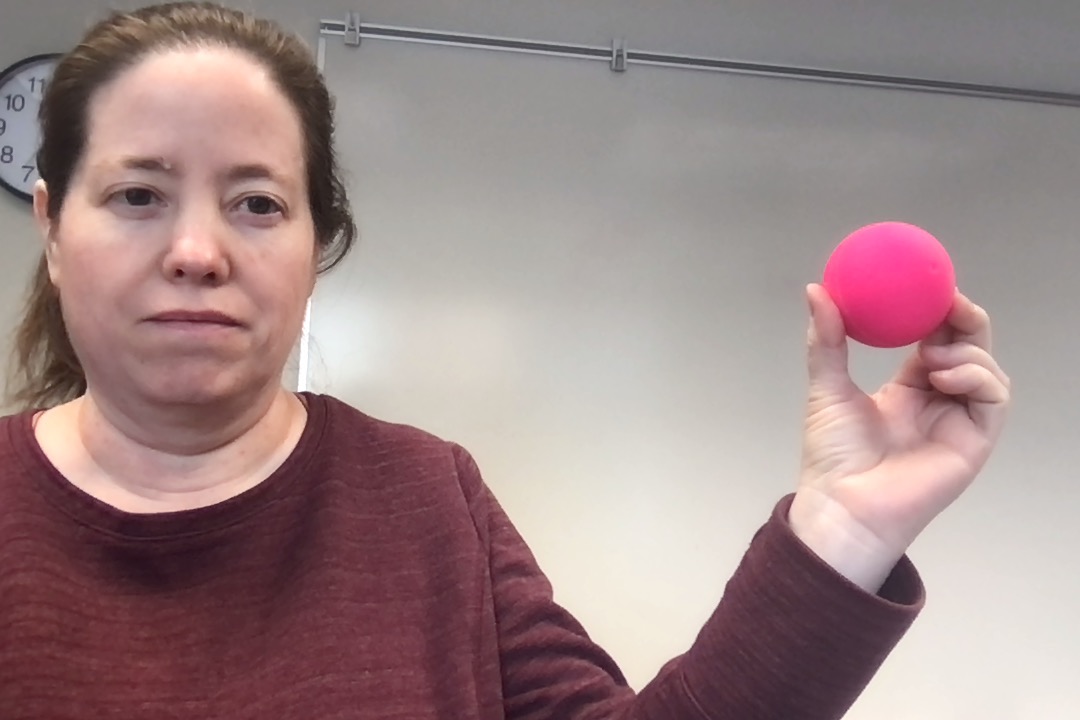
Figure 10 shows the original pink ball picture from BallFinding, along with a good ROI selected using the selectROI.py program.

5.2 Building a histogram of hues from reference image
The next step in the backprojection process is to build a histogram of hue values from the reference image. A histogram is used to count how frequently each range of hues occurs. Rather than having an entry for each possible value, we make bins that hold equal sized sequences of values. For instance, if we made 18 bins for the 180 hue values, then each bin would cover 10 hue values: bin 0 would count values between 0 and 9, bin 1 would count between 10 and 19, and so forth. (See Wikipedia article on Histograms if you don’t remember what a histogram is.)
Below is a code example that shows how to take a reference image and construct a histogram from it. You don’t need to understand the show_hist function right now: it takes a histogram (represented as a one-dimensional Numpy array) and it displays the histogram as a bar chart.
Code
import cv2
import numpy as np

def show_hist(hist):
    """Takes in the histogram, and displays it in the hist window."""
    bin_count = hist.shape[0]
    bin_w = 24
    img = np.zeros((256, bin_count * bin_w, 3), np.uint8)
    for i in range(bin_count):
        h = int(hist[i])
        cv2.rectangle(img, (i * bin_w + 2, 255), ((i + 1) * bin_w - 2, 255 - h), (int(180.0 * i / bin_count), 255, 255),
                      -1)
    img = cv2.cvtColor(img, cv2.COLOR_HSV2BGR)
    cv2.imshow('hist', img)
refImg = cv2.imread("referencePic.jpg")
cv2.imshow("Ref img", refImg)
histImage = cv2.cvtColor(refImg, cv2.COLOR_BGR2HSV)
hist = cv2.calcHist([histImage], [0], None, [18], [0, 180])
cv2.normalize(hist, hist, 0, 255, cv2.NORM_MINMAX)
hist = hist.reshape(-1)
show_hist(hist)
cv2.waitKey()- 1
- Convert the reference images into HSV format
- 2
- Calculate the histogram on the HSV image, looking only at the 0 channel (hue), with no mask, 18 bins, and values that range between 0 and 180
- 3
- Rescale the histogram so that the minimum value is 0 and the maximum is 255
- 4
- Change from a column vector (18 rows and 1 column), to a row vector (1 row, 18 values)
- 5
- Display the histogram as an image
The calcHist function is the most important, and complex, step in this code. It has five required inputs:
- First, it takes in a list of images, here we pass just one, but we have to pass it as a list containing one image.
- Second, we specify which channels of the image we want to build the histogram from (in this case just the 0, hue, channel).
- Third, we could pass in a mask, if we wanted to, but we pass in
Noneto indicate we don’t want to apply a mask. - Fourth, we specify the number of bins for the histogram (the function will divide the range of values as evenly as it can across the bins).
- Fifth, we specify the range of values, from 0 to 180 in this case.
Normalization, in computer vision, and in computer science more broadly, is the process of rescaling some collection of data so that the data values fall within a specified, canonical range. Here, we want to rescale height of the histogram data so that the maximum height of any bar is 255, and the minimum is 0. This will be needed for the next, and final, step, where we compute the backprojection.
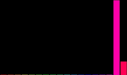
Figure 11 shows the histogram we would get if we selected a reference image for the ball in the earlier example.
5.3 Computing the backprojection
The backprojection algorithm treats the histogram we calculated as a probability distribution: the height of a bar represents the probability that the hues in that range match the reference image.
We apply this idea to our current image: for each pixel, we look at its hue and determine which bin of the histogram it falls into. We then use the value/height of that bin as the value in our backprojection image. The result is a threshold image, although often one with grayscale values as well as black and white. Pixels that match our reference hues are non-zero, with brighter pixels falling into the tallest bin.
The calcBackProject function takes in a list of images (they must be in HSV since our histogram is in HSV), a list of the channels to apply the backprojection to (just the hue channel, here), the histogram itself, the range of hue values, and an optional scaling factor, to modify the size of the output image.
Figure 12 shows the result of computing the backprojection using the histogram from the previous step.