In this chapter, we will take a closer look at how image representation works with OpenCV and Numpy, and tools from both libraries we can use to work with images. A key point to remember is that, though we can access individual pixel values, we will rarely ever write programs the manually iterate over the rows and columns of an image and read, or change, each individual pixel value. Doing so can be very slow. However, we can leverage the mathematics around vectors and matrices (a central focus of Linear Algebra) to treat images as matrices. This lets us use many highly-optimized algorithms for manipulating matrices, some of which leverage the multicore nature of modern computers.
The Numpy module implements N-dimensional arrays, a data structure that represents matrices, and it also provides those optimized algorithms for manipulating matrices. OpenCV sometimes has its own versions of basic matrix algorithms, as well.
1 Images as Numpy arrays
Images in OpenCV are represented as N-dimensional arrays from the Numpy module. Numpy (NUMerical PYthon) implements efficient data types for arrays of numbers, including the 2-d and 3-d arrays that we need to represent grayscale and color images. An image is a Numpy ndarray, and the individual numbers in the array are typically one of the special Numpy number data types.
Numpy implements its own number types, similar to types used in other programming languages such as C, C++, and Java. Each number type has these properties: integer or floating-point, signed or unsigned, and a bit-size. For instance, to represent color values we use an 8-bit unsigned integer (which can represent values from 0 to 255). There is a Numpy type, uint8, which is exactly this kind of integer. Numpy also provides larger integer types, signed integer types that can represent both positive and negative integers, and floating-point types, such as float32 (which holds signed 32-bit floating-point numbers).
Python, by contrast, has just one int and one float type, which can represent any integer or floating-point number that the computer can represent. How much memory an integer takes is hidden from us in Python, but Numpy makes that explicit to us. Similarly, Python lists are more flexible and fluid, and can be added to or removed from. Numpy arrays are less flexible: they hold just one type of number, and their size is fixed when they are created. These limitations allow them to represent data more efficiently, and increase the efficiency of accessing or changing data values.
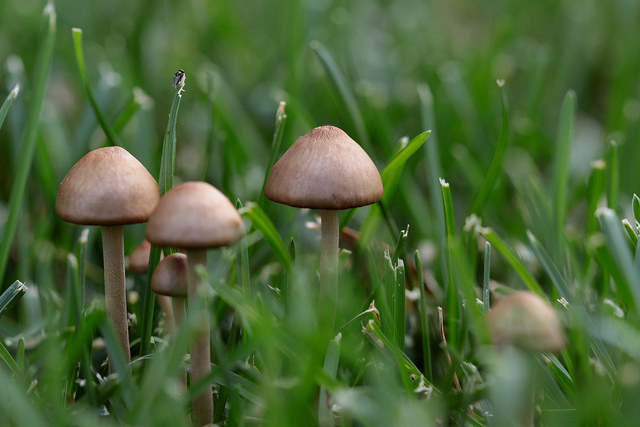
Figure 1: Mushroom image used in the next example, with 427 rows and 640 columns
The code example below reads in an image, and then prints its type, its size given as a tuple holding the size of each dimension of the array, and the type of data it contains. After that, it prints the array itself. Figure 1 shows the image that is used.
import cv2origImage = cv2.imread("Ch2-Images/mushrooms.jpg")print("Type:", type(origImage))print("Shape:", origImage.shape, " Data type:", origImage.dtype)print(origImage)
You can see that the actual type for the image is numpy.ndarray. Each Numpy array has some variables associated with it; we print two of them on the second line. The shape of an array is its size, given as a tuple with one entry for each dimension, given the length of that dimension. The dtype of an array is the data type: the kind of data stored in the array. Since images use 8 bits per color channel in the RGB/BGR format, and we denote those with only positive values (and zero), we want to use unsigned 8-bit integers for each value in the array: The Numpy type uint8 is exactly that.
When large Numpy arrays are printed, it automatically leaves out some of the data, putting in an ellipsis in each row and column where data has been omitted. It shows the first three elements and last three elements for each dimension: the first three rows and the last three rows, and within each row the first three pixels and the last three pixels. When we print a Numpy array it looks somewhat like a Python list, with nested brackets to show us the structure of the data. In this case, the outermost pair of brackets enclose the rows of the array. In other words, each element within the outer brackets is a row of the array. And each row can be thought of as an array itself. Within a row, each element is a color. And each color is itself an array of three integers. Those values are unsigned 8-bit ints.
To orient yourself with what has printed, consider the following hints:
The first row starts with the (0, 0) pixel in the upper-left corner of the image with color (34, 109, 65).
The last pixel in the first row has color (69, 108, 83).
The last row starts with color (44, 92, 66) and ends with color (34, 91, 53).
2 A few basic Numpy tools
In this section, we will introduce some basic functions, methods, and operations that apply to Numpy arrays. To keep examples simple, we will use small, simple arrays rather than images for many of these examples.
Whenever we want to use Numpy functions explicitly, we need to import the Numpy module. It has become standard to abbreviate the name of the module when importing it, so that it looks like the example below. Then, when using Numpy tools, we use the prefix np. rather than numpy..
import numpy as np
2.1 Creating an array
As we know, OpenCV will create an array to represent an image read from a file. But here we will examine some tools for creating arrays from scratch. More details about creating Numpy arrays may be found in the Numpy tutorial section Creating Arrays.
If we create a list or tuple with the structure we want in our Numpy array, the array or asarray functions can convert that to an array with the same structure. Each function takes one required input, the sequence or array to build the new array from, as well as optional inputs including dtype, which allows us to specify the type of data we want the new array to have. See the Numpy tutorial Data types for an extended discussion of Numpy data types, and how to specify them.
Below are some examples of making arrays with different structures with these functions.
We can also use these functions to copy an array and change the type of the data, etc. The array function always makes a copy of the data, while the asarray function, when given an array as input, may create a new view of the data, but not actually copy it. Thus changes to the original array can show up in the new array. We have seen a similar phenomena, aliasing, with shared data in lists. A Numpy array has a method astype, that can convert the contents of the array from one type to another. As with the asarray function, it may not copy the data, but rather just provide a view of it as a new type. (For an extended discussion of copying versus viewing, see the Numpy tutorial section Copies and view)
There are several functions to create arrays from scratch, by specifying only the size and data type. Each function fills the array with data that follows a particular pattern. We have already seen two of these functions, zeros and ones, but now we will look at them more closely. Additional functions include random.rand, which makes an array filled with random values, eye, which creates an identity matrix for any \(N\times N\) size, and arange, which fills the array with values where start and end are specified.
The zeros and ones functions take in a tuple that defines the shape of the new matrix to make. The most common optional input is dtype, where we can specify the type of data to put into the array. The zeros function makes an array of the given size, and fills each cell in the array with 0. The ones is similar, except that it fills each cell in the array with 1.
Numpy extends the built-in arithmetic operators to work on arrays. The four basic arithmetic operations, addition, subtraction, multiplication, and division, all perform element-wise operations on arrays. That means that it matches up corresponding elements of the arrays, and does the arithmetic on them. The examples below show this process on two arrays with the same shape.
We can always apply arithmetic operations when two arrays have the same shape. Numpy also allows us to perform arithmetic between an array and a scalar (an individual number). At each cell in the array, we perform the arithmetic on that cell’s value, and the scalar.
print(a1 +4)print(10* a1)
[[ 5  6  5]
 [ 8  9 10]]
[[10 20 10]
 [40 50 60]]
Numpy also allows arithmetic between two arrays of different shapes, if one can be naturally extended to map onto the other. It can be tricky to determine the rules for when something is extensible, but a simple case is when we have a 2-d array: we can specify a second array the length of a row and the arithmetic operator will extend that across all the rows of the array, and similarly for columns.
We can access and modify individual values in an array, or subarrays of various shapes and sizes, using an extended version of the square bracket notation Python uses for lists and strings, as well as an extended version of slicing. Numpy’s introductory tutorial has a section, Indexing on ndarrays, that goes into more details about accessing and indexing.
If we have a one-dimensional Numpy array, holding data in a single row, then accessing its elements or slicing out a subarray looks just like operating on a list.
Suppose we have a two-dimensional array. Its structure matches that of a nested list. With nested lists, a single square bracket returns the whole nested sublist. To access an individual value inside that sublist, we add a second square bracket (see first examples below).
With a two-d array, a single square bracket with a single number returns the subarray corresponding to that row. We can add a second square bracket after the first, with a similar effect as with lists, but Numpy also allow us to put both indices inside a single pair of square brackets, separated by commas. This is an easier notation (see second examples below).
List element: [7, 6]   Sublist element: 7
Array element: [7 6]   Subarray element: 7   and simpler notation: 7
We can always replace the single number with a slicing operator, where we specify start and end indices, and step size, to select a range of values from an array. Notice that we can use a single colon (:) to indicate all values for a given dimension. Remember that if we leave out start or end then Python assumes it should start at 0 and go to the end of the current dimension. And if we have two colons, the value after the second colon is a step size or number of elements to skip. Before looking closely at the output for the examples below, try to predict the output for the random array shown here and the code below.
print("Selecting just rows 2 through 4:")print(rArr[2:4])print("Selecting all rows of columns 0 and 3:")print(rArr[:, ::3])print("Selecting rows 2 and 3 and columns 2 and 3:")print(rArr[2:4, 2:4])print("Selecting the last value from all rows:")print(rArr[:, -1])
Selecting just rows 2 through 4:
[[39 35 88  0 58 23]
 [53 41 12 11 51 73]]
Selecting all rows of columns 0 and 3:
[[10 51]
 [60 52]
 [39  0]
 [53 11]
 [61 85]
 [47 83]]
Selecting rows 2 and 3 and columns 2 and 3:
[[88  0]
 [12 11]]
Selecting the last value from all rows:
[ 8 62 23 73 99 40]
We use slicing like this on images to extract a rectangular region of an image, called a region of interest (ROI). See discussion in a later section.
2.4 Using boolean arrays
The last Numpy tools we will look at are boolean arrays. These arrays allow us to apply comparison operations to whole arrays, creating arrays the same shape filled with True and False. We can use Numpy functions any and all to ask whether the resulting array has any true values, or if all are true values.
Most exciting, we can use boolean arrays as a selection index inside square brackets, to extract just the values from the array where the boolean array has True. (Much more can be found in the Indexing with boolean arrays section of the Numpy quickstart guide.
As we saw in the previous section, Numpy provides arithmetic operations on arrays. OpenCV provides its own set of functions to perform arithmetic on images. We might prefer Numpy’s operations for their simplicity in terms of writing code, and also probably a slightly better speed, but the Numpy operations can have some bad effects, and OpenCV’s arithmetic functions are safer.
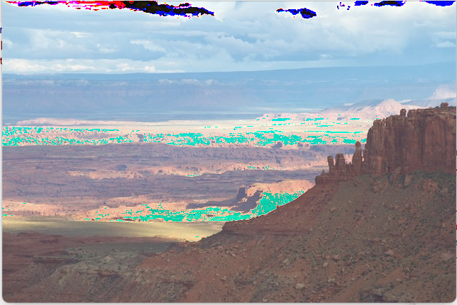
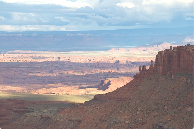
Consider the code example below. It is brightening an image by adding 50 to each value in the array (all three color channels, every rown and column). The results are shown in Figure 2.
Figure 2: Comparing arithmetic effects of Numpy and OpenCV
In this example, the Numpy arithmetic leads to strange color artifacts in the resulting image. Why? This is an example of overflow. With an unsigned 8-bit integer, the largest value we can represent is 255. If we add 50 to a number like 235, the result should be 285, but we can’t represent that in 8 bits, so the result wraps around to the bottom of the range, giving the value 29. The color artifacts occur when some or all color channel values overflow. When the result looks black or dark gray, then all three channels overflowed. If the result looks red, then both blue and green overflowed, and so on.
Numpy arithmetic does not check for or correct for overflow!
If we use Numpy arithmetic, it is our responsibility as programmers to ensure that overflow can’t happen.
On the other hand, OpenCV’s arithmetic function doesn’t show these artifacts. This is because it checks if overflow might occur, and if so, it sets the channel value to 255. This makes it more safe, more reliable, but that extra check also means it will run slightly slower than the plain Numpy version.
To learn more about Numpy, check out the Numpy documentation. And for more about OpenCV’s arithmetic operations, see OpenCV’s Operations on arrays documentation.
4 Accessing color channels
Remember that color images in OpenCV are, by default, represented as BGR 3-d arrays, where the first and second dimensions are for rows and columns of pixels, and the third dimension holds the three color channels in blue, green, and red order. There are times when we want to separate the channels from each other, perhaps to brighten only the blue channel, or reduce the amount of red. We can use the slicing operators from the previous section to slice out the channels for each other.
But OpenCV provides us with a function, split, to separate the channels into their own arrays, as well as a function, merge, to put channels back together again. The split function takes one input, a color image, and it returns a tuple of the three channel arrays. The merge function takes a tuple containing three channel arrays (each must be a 2d array, and all the same size) and it returns a new image array.
The code example below splits the channels of an image, and then copies and modifies two of the channels: one with increased blue, and the other with decreased red. Finally, the code merges the three channels back together again to create two new images and displays them. Figure 3 shows the original image and the two with modified color channels.
Figure 3: Examples of splitting and merging to change color channel arrays
Note that we can make channel-specific changes using Numpy’s tools as well, though we may run the risk of visual artifacts. Figure 4 shows what would happen if we used Numpy. Notice that increasing the blue works well, because blue values were generally not high, but reducing red, for pixels that had little red to start with, causes overflow.
Figure 4: Examples of using Numpy arithmetic to change channel values
5 Regions of interest
When working with images, especially in the context of computer vision, we often want to isolate and focus on smaller section of the overall image. We call these sections “regions of interest” (ROIs). We can treat them as smaller images in their own right.
To create a region of interest, we can use Numpy’s slicing operators to select a certain range of x and y values from an image.
Note: for memory efficiency, when you create an ROI, it is a new view on the original image data. It does not copy the data. Many times this is just what we want: we can focus on a small section and any changes we make show up in the original. However, when you are working with a view onto a different image, some operations are prohibited (for example, you are not allowed to draw on an ROI that is a view). You can always use the copy method to explicitly make a copy of the data, working with a real, new image.
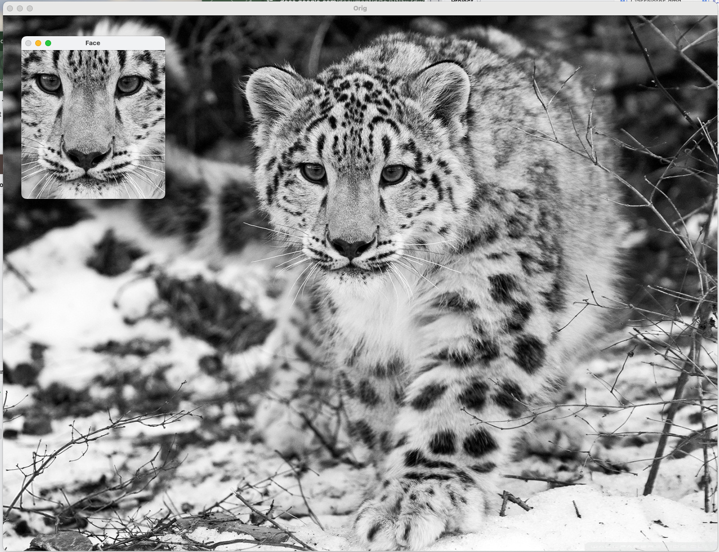
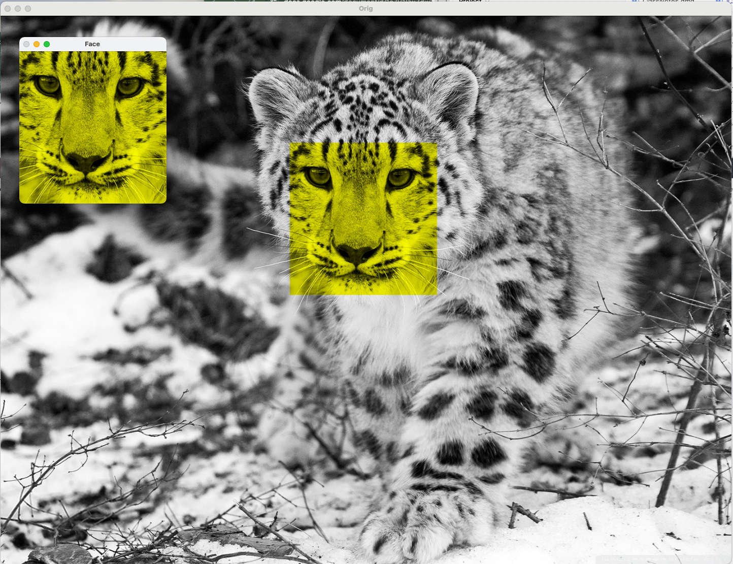
The code below illustrates how to make an ROI, and what happens when you manipulate it. This code reads in one of the snow leopard images, and defines an ROI faceROI that is centered on the cat’s head (the actual coordinates for the ROI were found with trial and error). It changes the blue channel values for the ROI to be zero, which will also change the original image (you must call imshow again to see the changes).
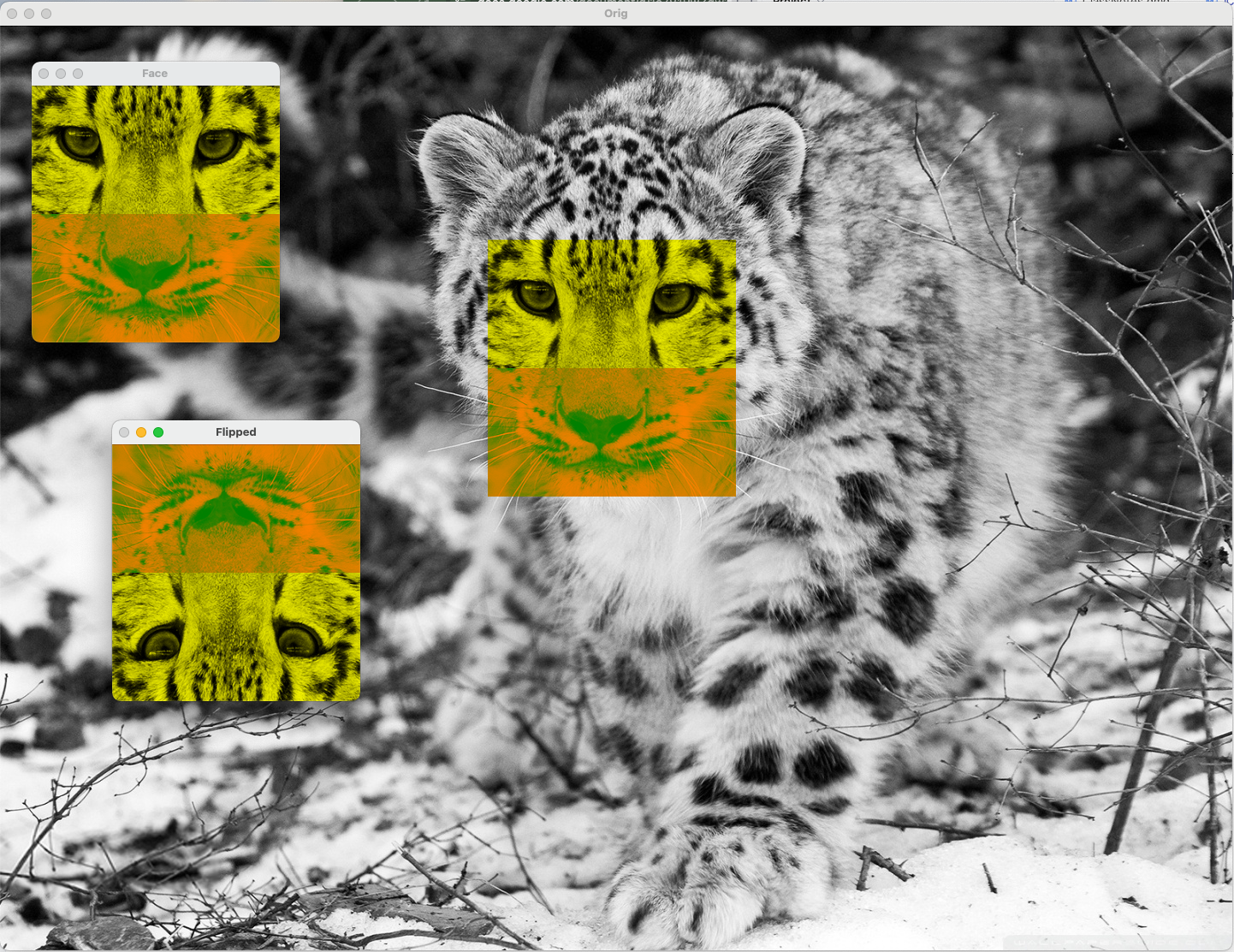
Finally, this program creates a second ROI, where we have reversed the rows in the y direction, so that it is upside down from the original. We then change the green channel values for the second ROI to be 128, and view the original images again. Run this script on your own computer; the results are shown in Figure 5 below.
import cv2catImage = cv2.imread("SampleImages/snowLeo1.jpg")faceROI = catImage[250:550, 570:860, :]cv2.imshow("Orig", catImage)cv2.imshow("Face", faceROI)cv2.waitKey(0)# set blue channel of this ROI to zero, notice change shows in originalfaceROI[:, :, 0] =0cv2.imshow("Orig", catImage)cv2.imshow("Face", faceROI)cv2.waitKey(0)# flip the face upside down by reversing the Y direction and keeping the others the sameflipFace = faceROI[::-1, :, :]hgt, wid, dep = flipFace.shape # get dimensions of ROIflipFace[:hgt//2, :, 1] =128cv2.imshow("Orig", catImage)cv2.imshow("Face", faceROI)cv2.imshow("Flipped", flipFace)cv2.waitKey(0)
Original image and first ROI
Changing first ROI blue values to zero
Creating flipped ROI and changing green values to 128 in its top half