1 Getting started with OpenCV
OpenCV is an add-on module in Python. Modules contain constants and functions that have a special purpose. They are not automatically loaded and available when we start up the Python interpreter. We have to explicitly ask for them to be loaded using the import command. For instance, the command below will load the OpenCV tools.
You can type the import command into the Python shell, or you can put it in a script file.
Note: Always put all import statements at the top of your file.
There are many useful modules provided by Python, or added by third-party developers. Other modules you might explore include math, random, statistics, sys, and os. A secondary module used by OpenCV is numpy, which provides efficient tools for representing and manipulating multidimensional arrays of numbers.
When you import a module, Python makes a special separate namespace where the tools from that module reside. In order to access them, you must tell Python to look in that namespace by attaching the name of the module, followed by a period. You’ll see examples of this below.
In Python, the OpenCV module is called cv2.
OpenCV has excellent online documentation, and you will need to become familiar with using it (as discussed in Chapter 0).
Try examples! Throughout this and future sections, you are encouraged to try the code examples along with the reading. To prepare for that, set up a project in PyCharm using the version of Python that has OpenCV installed in it, and move a copy of the SampleImages folder into the project. Put your code files in the top level of the project, alongside the SampleImages folder.
1.1 Reading and displaying images
import cv2
img1 = cv2.imread("SampleImages/snowLeo1.jpg")
cv2.imshow("Leopard 1", img1)
img2 = cv2.imread("SampleImages/snowLeo2.jpg")
cv2.imshow("Leopard 2", img2)
cv2.waitKey(0)- 1
- Load the OpenCV module
- 2
-
Read in the image from
snowLeo1.jpg, assignimg1to hold the image - 3
-
Display the image in
img1with titleLeopard 1 - 4
-
Read
snowLeo2ljpgintoimg2and display it asLeopard 2 - 5
- Wait for the user to hit a key before continuing
Note about paths: In Chapter 0 we discussed the importance of understanding paths in order to write programs that work with files. When we read in an image file, we must specify an absolute or relative path that is correct, as well as spelling the filename correctly. For this to work, you must configure your project so that:
- The
SampleImagesfolder is in your project folder - The code file you make is in the same project folder as
SampleImages(not insideSampleImagesitself!)
The relative path used in the code above starts from the folder where the code file is, and tells the computer how to navigate from there to where the image file is.
Copy this program and run it to see what happens. You should see two windows pop up, showing the two snow leopard images (they may appear under other windows). To get the program to finish, click on one of the image windows to make it active, and then hit a key on the keyboard. The window should disappear and PyCharm should be done with the program.
OpenCV uses the string that is the first input to imshow to identify windows: if you use call imshow again with the same string but a new image, the new image will appear in the same window. To see this, change the string for the second imshow above to be "Leopard 1". Then rerun the script. You probably will not see the first image, because it is overwritten so quickly by the second one. To slow things down, copy the waitKey line and put it right after the first call to imshow.
1.2 Color representations
Colors we perceive in the real world derive from different frequencies of light emitted or reflected off objects in our world, and filtered through our brain’s perception systems. Color theory is an extremely interesting field of study, with contributions from mathematics, physics, biology, art, photography, psychology, and more.
Inside the computer, we must convert color into a discrete, compact representation: a digital representation. There are dozens of ways of representing color digitally, though a few are most common. Below, we will explore several common color representations used to represent images.
1.2.1 RGB color representation
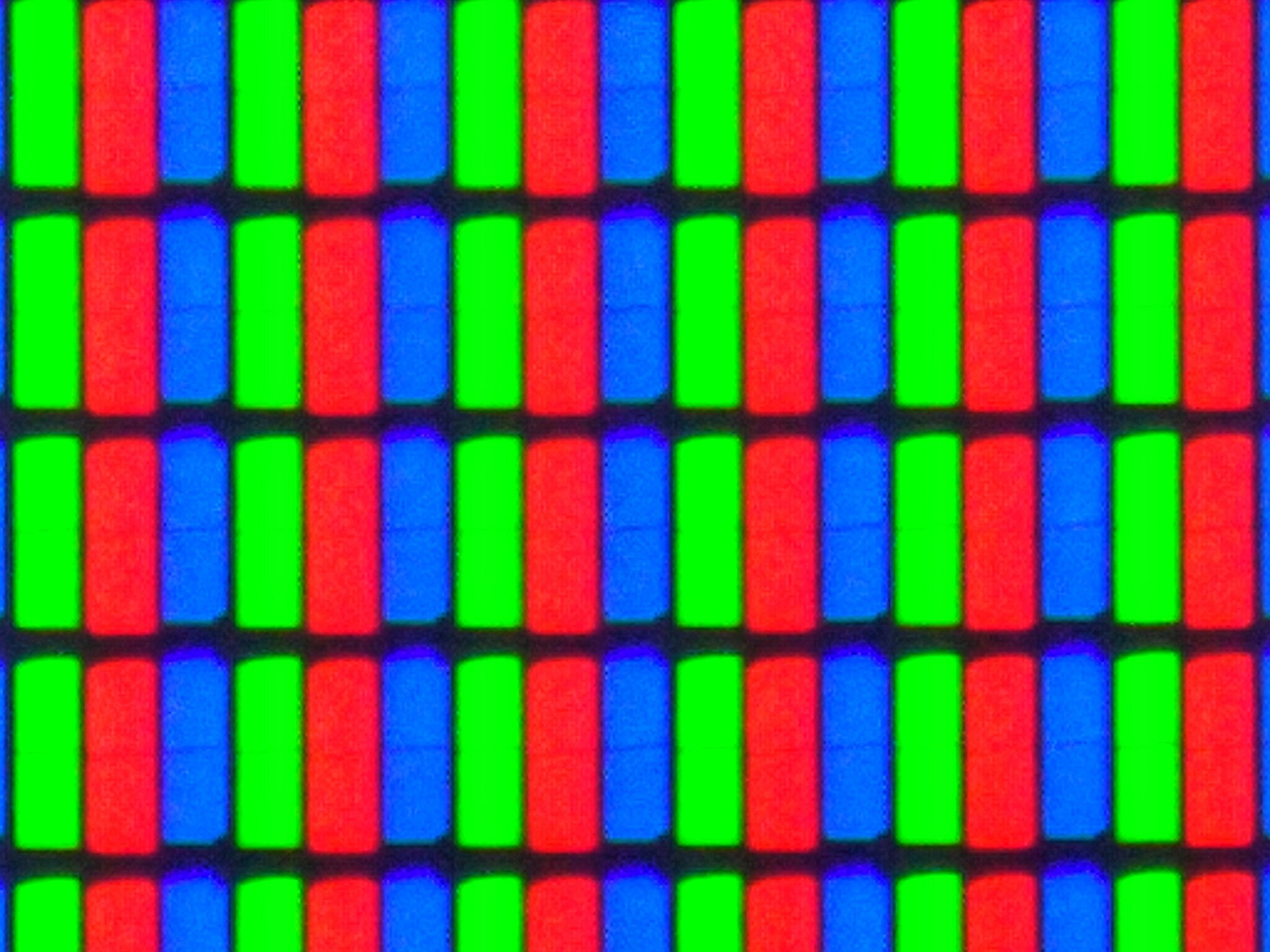
The most common representation of colors for images is the RGB (red, green, blue) format. This is because monitors and projectors typically use RGB to display colors to us. If you have ever looked closely at a projector’s output, or looked at a droplet of water on your phone screen, you can see dots of red, green, and blue light very close together (see Figure 1).
Long ago, pointillist artists discovered that small dots of color close together can fool the human eye into perceiving a different color altogether. Similarly, photographers from the 19th century figure out that they could simulate color photos by layers three copies of a photo together, one tinted with red, one with green, and one with blue. Only later did scientists come to understand how human color vision works, and why these methods work for us.
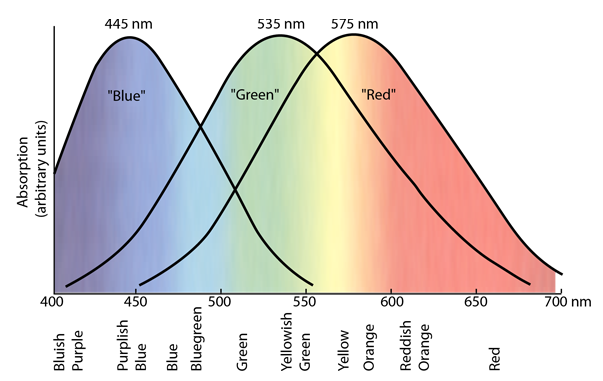
In human eyes, we have three different color receptors, or cones. Each kind responds to a different range of wavelengths, and responds more or less strongly depending on the wavelength (see Figure 2). If we display red, green, and blue light in close proximity, the human eye can be fooled into perceiving a corresponding wavelength of light.
In the RGB color representation, we call the three values of red, green, and blue light channels. We represent colors as a collection of three values, one for each channel. A good metaphor for how RGB works is that we have three sliders as shown in Figure 3, one for each channel, and we can move them independently to select a different amount of light. The result is the actual color we are representing.
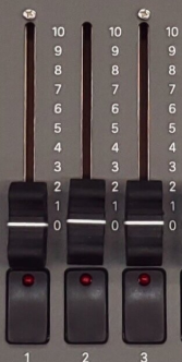
The position of the slider indicates how much of that channel’s light we are mixing. Shades of gray occur when all three channels have the same value. Black is the absence of all light, and white is full power to all three channels.
Sliders that control lights typically vary continuously in the positions they can take. However, inside the computer we need things to be discrete, so one question that arose is: how many different values do we need for each channel to get photorealistic images? If each slider was actually a light switch, it would have just two positions: on and off. We can represent these as 1 and 0. The table below shows all the combinations of the three switches, and the colors they correspond to.
| R | G | B | Color |
|---|---|---|---|
| 0 | 0 | 0 | Black |
| 0 | 0 | 1 | Blue |
| 0 | 1 | 0 | Green |
| 1 | 0 | 0 | Red |
| 0 | 1 | 1 | Cyan |
| 1 | 0 | 1 | Magenta |
| 1 | 1 | 0 | Yellow |
| 1 | 1 | 1 | White |
Obviously, we want more than just two values per channel, but this representation only requires three bits of information inside the computer.
Side note on binary representations: All data inside a computer is ultimately represented in binary, as a sequence of ones and zeros, because computers use the presence or absence of electricity in a wire, or the direction of a magnetic field, to represent data. A bit is the smallest unit of information: zero or one, (yes/no, true/false, on/off). Modern computers almost all use a collection of 8 bits as the smallest useful unit of data: this is called a byte (4 bits is called a nibble, computer scientists like puns!). When we are choosing how to represent data, sometimes we must consider how many bytes that data will take up.
There is an important relationship between the number of bits in a representation, and how many distinct patterns or values we can represent. If we have \(k\) bits in our binary representation, then we can represent \(2^k\) distinct values. Above, we had 3 bits per color: there were \(2^3 = 8\) binary patterns, corresponding to eight distinct colors.
Representing colors by their frequencies or wavelengths might need an 8-byte floating-point number. Representations based on multiple channels, each holding integers, can be more efficient.
The typical representation for RGB channels provides one byte (8 bits) for each channel, for a total of 3 bytes to represent a color. According to the rule above, each channel can represent \(2^8 = 256\) distinct values: 00000000, 00000001, 0000010, … 11111110, 11111111. We use nonnegative integer values starting with zero; we call this kind of number an unsigned integer. In the case of color channel values, we use the integers from 0 to 255. The total number of distinct colors we can create with this representation is \(2^{24} = 16,777,216\), more than 16 million distinct colors!
We represent a color as a collection of three 8-bit unsigned integer values, one for each channel.
There are many online “color pickers” that let us generate colors, and shows us the color representations in different formats. Explore the color picker at HTML Color Codes. Because this is designed for choosing web colors, it shows each color in a Hex representation, in RGB, and in HSL. The Hex representation is used on websites and other applications for colors: it is actually the RGB color values, rewritten into hexadecimal (base 16) notation (to see this, click on a color close to black, where the values will be close to zero). Notice that the RGB values are always in the range from 0 to 255.
HSL stands for “hue, saturation, lightness” and is a very different color representation than RGB. We will not use HSL, but it is closely related to a color representation called HSV, which we will use when using color to segment images or track objects. (See HSL and HSV, Wikipedia for more details about how HSL and HSV relate.)
OpenCV in Python chooses to represent RGB colors backwards, as BGR. That means that a color is a tuple containing three numbers: blue channel, green channel, red channel. A tuple is like a list, but can’t be modified. The numbers in the tuple must be integers between 0 and 255. For instance, Figure 4 shows three colors and their BGR representations in OpenCV


1.2.2 Other color representations
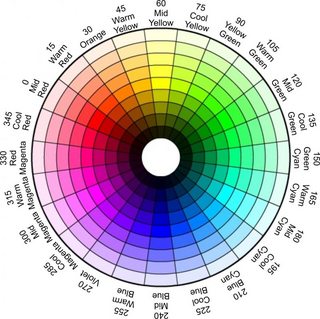
There are many other color representations that we could use. As mentioned before, one used for color-based algorithms is called HSV (hue, saturation, value). In HSV, the basic color is defined by single channel value, the hue. Hue values are interpreted as degrees around a circle: 0 to 359. The other two channel values are thought of as percentages, often in the range from 0 to 100.
The saturation channel describes how “pure” or intense the color is: one way to think of saturation is how mixed with white the color is: high saturation values have little mixture with white, low saturation are strongly mixed with white. The value channel captures the brightness of the image: you can think of it as changing values appear mixed with white or gray. The value defines the color’s brightness, changing the shade of gray that we mix into the saturation: low values cause the hue to be mixed with dark gray or black, high values mix with light gray or white. The colorizer color picker, while more clumsy to use, does include HSV as one of its options (also called HSB). Figure 5 shows the mapping of hue values to degrees in HSV.
HSV is useful for color-tracking in images, because the hue changes relatively little when the brightness of the light changes, whereas all three channels in an RGB image change when the brightness changes.
OpenCV represents HSV values as a tuple of three 8-bit unsigned integers, much like RGB. That means the values are limited to the range from 0 to 255. How does that work when the usual ranges of HSV values are 0-360, 0-100, and 0-100?
- The hue channel in OpenCV uses the range from 0 to 179, dividing the HSV degrees in half. Thus, a midgreen value in Figure 5 above normally has value 120: in OpenCV we use 60 for this hue instead.
- The saturation and value channels normally runs from 0 to 100. OpenCV rescales them to range from 0 to 255. To convert a “global” saturation level to OpenCV, use this formula: \(s_{opencv} = \frac{s_{global}}{100} \cdot 255\).
On beyond HSV
There are many additional color representations, each with its own strengths and uses. As one example, the YUV color representation has three channels: YUV. The Y channel contains brightness or “luminance” information, and the U and V channels together describe the color. We use this color representation for balancing the brightness of an image, by converting to this format, modifying the Y channel, and then converting back to BGR for display/use. The YUV Colorspace web page gives some nice visuals showing how this representation works.
1.3 Image representation
Given a specific color representation, we now have to figure out how to represent a whole image. We want to distinguish between how an image might be represented when stored as a file, and how it might be represented when read into a program. In both cases, multiple representations are possible, though for our purposes we don’t need to know the details of different file representations, and we will focus on OpenCV’s method for representing images.
When an image is stored in a file, the file format often keeps the image’s data in a compressed form, saving space. The exact format and kind of compression used is signaled by the file extension (.jpg, .png, .gif, etc.). OpenCV can work with many file formats, but the extension must match the actual contents for any program to be able to read or display an image. Don’t just change the extension: that will just make the file unreadable. You have to use a program to convert from one representation of an image to another, if needed.
Once an image is read into a program to be manipulated, however, the image representation is very different from that in a file, and images are represented the same way, whether they originated in a jpg or png or any other file format. Different programming tools use slightly different representations for images, but all share certain key features:
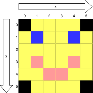
- An image is a grid of pixels (short for picture elements)
- Each pixel contains a single color
- We interpret the horizontal dimension of the grid as the x dimension, with 0 at the left, increasing to the right
- We interpret the vertical dimension of the grid as the y dimension, with 0 at the top, increasing downward
- Locations for specific pixels are given as (x, y) coordinates
Figure 6 shows a tiny, 6 pixel by 6 pixel image, with x and y dimensions and indices given. The blue pixel representing the right eye is at (4, 1).
Note that a pixel is not a unit of measurement. While image files often store a mapping between numbers of pixels and distance, such as ppi (pixels per inch), that is not an intrinsic property of the images. A pixel is simply the smallest unit of an image. When the pixels are drawn small enough, we don’t notice the individual pixels, and instead see the whole picture. #fig-showPixels shows the “Mighty Midway” picture from SampleImages, and then a portion of the picture, zoomed in far enough to see the individual pixels. The original picture is 1000 pixels wide by 667 pixels tall.
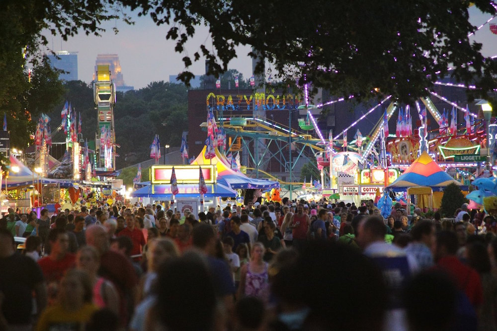
mightyMidway.jpg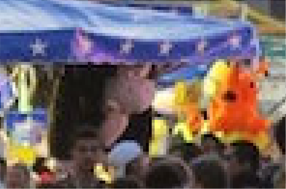
mightyMidway.jpg image, and a section zoomed in to show pixels
Grayscale versus color images
There are three variations on images: color, grayscale, and black-and-white. We have discussed color images and how color might be represented already. Grayscale images contain only shades of gray between black and white. As we noted earlier, shades of gray correspond to the RGB channels holding equal values: (195, 195, 195) is a medium bright shade of gray. Black-and-white images contain only black pixels and white pixels, no shades of gray in between.
Because a grayscale image has equal channel values, we only need to represent one copy, the luminance or brightness (for the gray shade above, just one 195 is needed). OpenCV represents grayscale images as a two-dimensional array, or matrix, of numbers. In Figure 8 a small example of a grayscale image is shown on the left, with
Color images, however, have more data per pixel, and generally use 2-4 numbers to represent each color. In OpenCV, we represent this by using a three-dimensional matrix: the first dimension is x, the second dimension is y, and the third dimension is for the channels. Figure 8 illustrates the structure of an OpenCV color image.
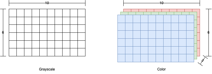
Images in OpenCV are represented using Numpy arrays: we will return to this subject later when we look more closely at the Numpy module and the tools we may use to manipulate image arrays.
1.4 Drawing with OpenCV
OpenCV provides a set of tools that allow you to draw shapes on images. We can also make blank images to serve as “canvases” for our drawings. In this section we will explore the different drawing functions OpenCV provides, and you will also learn how to save an image to a file, so you can store the results.
1.4.1 OpenCV drawing commands
In this section we will introduce the basic drawing commands, and their basic inputs. You can find more commands and more details in the Drawing Functions page of the OpenCV documentation; each function has more optional inputs than are given here.
In each example below we will use the same set of variables as is used in the documentation:
imgis a typical OpenCV image, a Numpy arraypt,pt1, andpt2are all points, tuples containing x and y indices into the imagecoloris a color, a tuple containing blue, green, and red valuesthicknessis line thickness, how wide to draw the lines, and if negative then the shape is drawn “filled-in”angle,startAngle, andendAngleare all angles, typically between 0 and 360, though other angles may be permitted
Note: Drawing or making other changes to an image does not automatically update the image displayed previously by a call to imshow. You must call imshow again to see the changes.
Drawing lines
The line function takes in an image to draw on, two (x, y) coordinate points, input as tuples, and a color (given as a BGR tuple). The thickness input is optional, but is often used to tell how many pixels wide the line should be. If you do not specify thickness the line is drawn as one pixel wide. The function draws a line as specified between the two coordinate points.
Drawing rectangles
The rectangle function takes in an image to draw on, and two (x, y) coordinate points, as tuples. Typically, we also specify the color tuple and line thickness. The two points specify two opposite corner pixels of the rectangle to draw (for instance, upper-left and lower-right corners). If the line thickness is 1 or greater, then a line rectangle is drawn with the given corner points, line color, and line thickness. If the line thickness is negative then a filled in rectangle with the given corners and color is drawn.
Drawing circles
The circle function takes in the image to draw on, the center point of the circle (a pixel location as an (x, y) tuple), an integer radius for the circle, and a color tuple. Line thickness is optional, and works the same as for rectangles: positive specifies line thickness, negative draws a filled-in circle.
Drawing ellipses
Drawing ellipses (ovals) is the most complicated of the functions we will look at, because the function not only draws ellipses but also arcs and partial ellipses, both line and filled. Therefore, we will go into more details about what each input parameter does.
To take the easy ones first, img is the image to draw on, pt is the center point as (x, y) coordinates (if you like mathy details, pt is the center point of the circle that circumscribes this ellipse, as ellipses are usually defined by two points). The color and thickness inputs work just as for the other drawing commands.
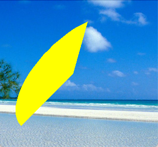
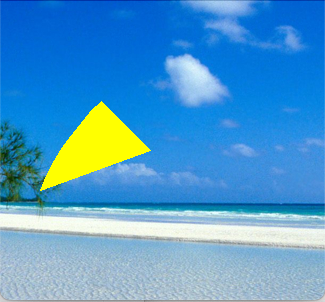
For the remaining inputs, we will illustrate them with a specific example, shown below.
import cv2
beachIm = cv2.imread('SampleImages/beachBahamas.jpg')
cv2.ellipse(beachIm,
(500, 250),
(70, 150),
45,
0,
360,
(0, 255, 255),
2)
cv2.imshow("Beach", beachIm)
cv2.waitKey()- 1
-
img, the value ofbeachIm - 2
-
pt, a tuple holding the (x, y) center point - 3
-
axes, a tuple holding sizes of ellipse’s axes - 4
-
angle, an integer angle, rotated from the horizontal - 5
-
startAngle, an integer angle, where to start drawing ellipse arc/wedge - 6
-
endAngle, an integer angle, where to stop drawing ellipse arc/wedge - 7
-
color, the color for the ellipse - 8
-
thickness, line thickness or to make ellipse filled
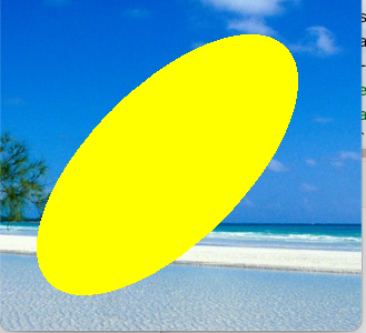
This program produces the ellipse shown in @figure-ellipse0.
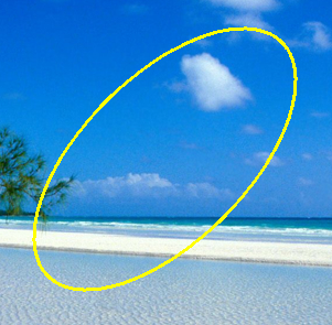
The axes input specifies the width and height of the ellipse in the form (r1, r2). To interpret these, first think of the ellipse as being unrotated. Then its first axis is horizontal, and the second axis is vertical. The r1 value is one-half the length of the first axis, and r2 is one-half the length of the second axis. Figure 10 show the (x, y) center point, and the length and meaning of the axes tuple (r1, r2).
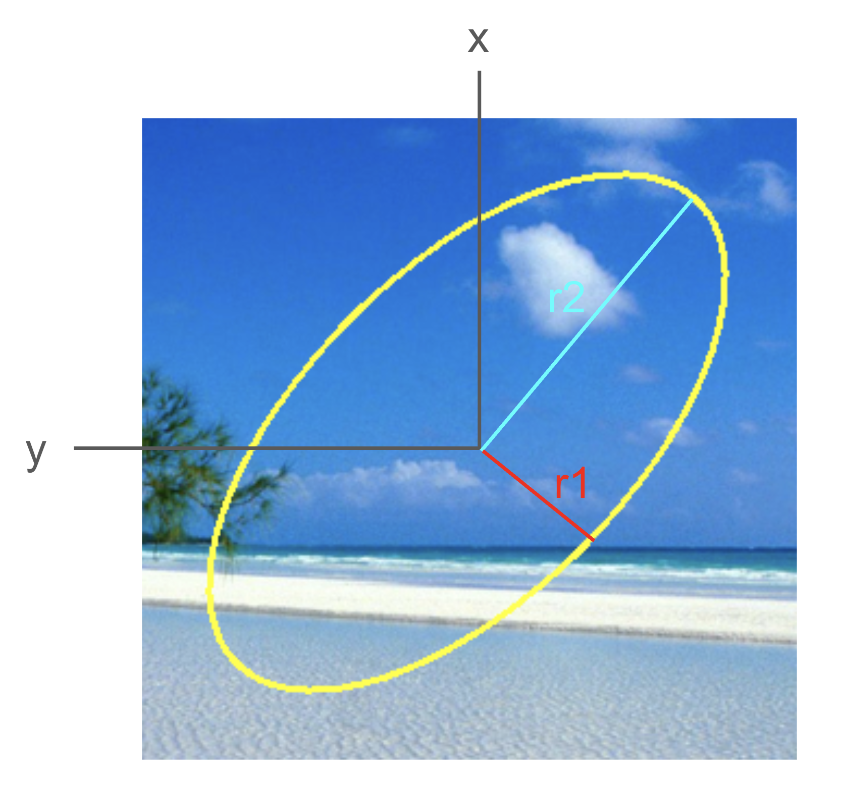
In this code example, the total width of the ellipse along its first axis is 140 pixels, and the total height of the ellipse along its second axis is 300 pixels.
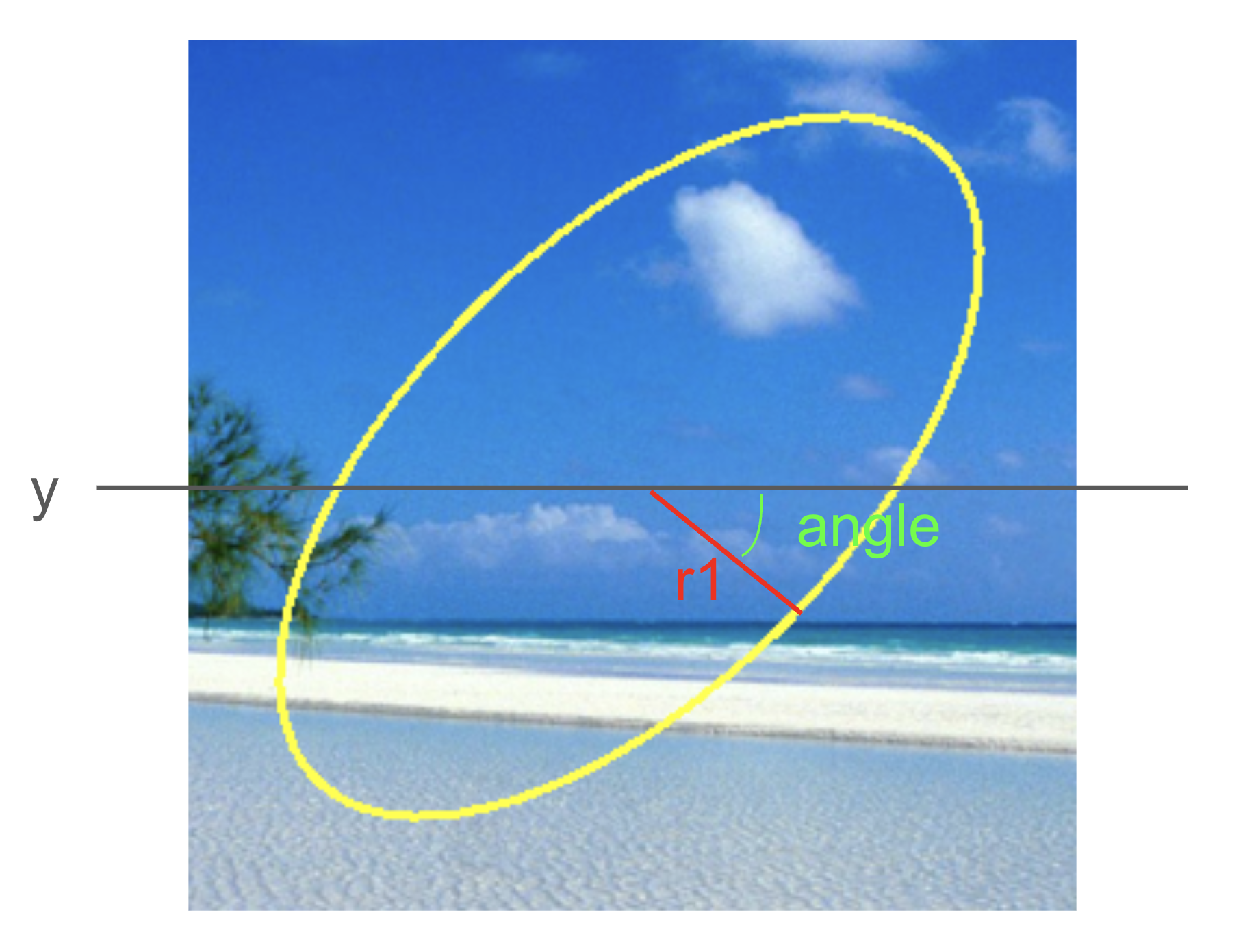
The angle input specifies how far to rotate the ellipse in the clockwise direction from a start where its first axis is horizontal. Another way to think about it is that angle is the angle between the horizontal and the first axis. You can pass negative angles here, to get counter-clockwise rotations. Figure 11 Shows how angle is determined for our example.
The last two inputs to discuss are startAngle and endAngle. We will start with a simple rule: when in doubt, set startAngle to 0 and endAngle to 360. This will draw the full ellipse.
You only need to vary startAngle and endAngle if you want to draw just a portion of the outline of the ellipse, or a wedge of the filled-in ellipse. In those cases, you need to understand how they work.
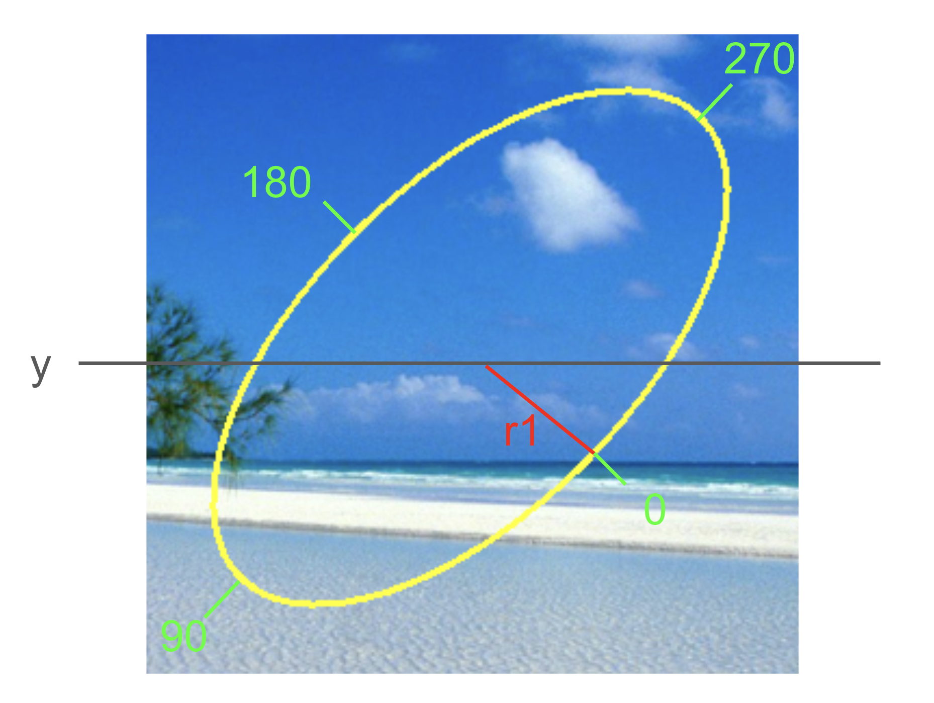
Imagine that the computer, in drawing the ellipse, starts at the end of the first axis on the right side of the ellipse, and draws the ellipse in a clockwise manner, ending back where it started. When drawing a partial ellipse, the computer follows the same path, but holds the (metaphorical) pen above the paper, except where specified by the start and end angles. Between them, startAngle and endAngle specify where on the rim of the ellipse to start drawing the ellipse, and where to end drawing the ellipse.
Each of these angles takes on a value between 0 and 360, where 0 is the right-side first-axis point, and the others rotate around the ellipse clockwise. !fig-ellipse3 shows the locations for 0, 90, 180, and 270 for our example ellipse.
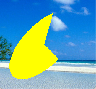
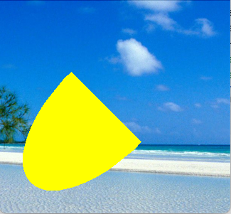
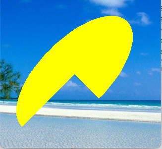
!fig-partialExamples shows nine pictures of an ellipse similar to the one shown above, but drawn as a filled ellipse. Each is labeled with the values for startAngle and endAngle used to create it.
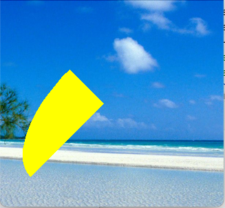
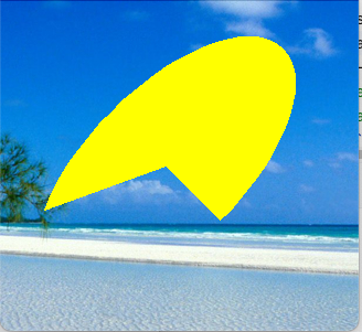
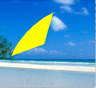
Be prepared to experiment any time you want to use the ellipse function.
Adding text to images
OpenCV can draw text on images, though the tools, and fonts, are rather bare-bones. The inputs include the image to draw on, the text to draw, and a point tuple specifying where to draw the text, plus the font, scale of font, text color, and line thickness for the text.
The point tuple gives the pixel where the lower-left corner of the text will appear.
The font is chosen by selecting from OpenCV’s built-in basic fonts (you are welcome, even encouraged, to explore how to add and access additional fonts on your own). By default, OpenCV includes a subset of the Hershey font family, shown in the table below
| Font Name | Description |
|---|---|
cv2.FONT_HERSHEY_SIMPLEX |
Normal-sized sans-serif font, simple complexity |
cv2.FONT_HERSHEY_PLAIN |
Small-sized sans-serif font, simple complexity |
cv2.FONT_HERSHEY_DUPLEX |
Normal-sized sans-serif font, medium complexity |
cv2.FONT_HERSHEY_COMPLEX |
Normal-sized serif font, medium complexity |
cv2.FONT_HERSHEY_TRIPLEX |
Normal-sized serif font, high complexity |
cv2.FONT_HERSHEY_COMPLEX_SMALL |
Small-sized version of COMPLEX font |
cv2.FONT_HERSHEY_SCRIPT_SIMPLEX |
Handwriting font, simple complexity |
cv2.FONT_HERSHEY_SCRIPT_COMPLEX |
Handwriting font, medium complexity |
The fontScale input is a floating-point number. It can be set to 1.0 to use the default size. Values greater than 1 will draw the font larger, values between 0.0 and 1.0 will shrink the font, and negative values will draw the text backwards!
1.4.2 Writing images to files
When we modify images in Python, the changes are only to the copy of the data that we have loaded into our Python program. They are not saved to the original file we read in. This is probably wise!
That said, you might create a beautiful picture and want to save it to a file. You can do that using the imwrite function. Always use a new filename when saving an image to file. Beware! if you use an existing filename in imwrite, you will overwrite the previous contents of that file
You call imwrite and first give it a path and filename where you want the new image to be saved. Be sure to include the extension, otherwise OpenCV does not know how to format the image data correctly in the file. The second input to imwrite is the image array itself.
1.4.3 Simple Drawing Example
The script below creates three images, and then illustrates each of the new images from scratch and then illustrates each of the drawing functions; it saves the resulting pictures to two files. It uses two numpy commands: zeros and ones. The zeros function makes an n-dimensional matrix filled entirely with zeros. In this case, we give the dimensions we want (300 rows, 500 columns, 3 channels) and tell it to make the numbers be uint8, the special type we need for 0 to 255 values. The ones function makes a matrix filled with ones. This call has 500 rows, 300 columns, and 3 channels, all filled with uint8. Copy these commands into a script and run it. Note that the imwrite function saves an image to a file. The type of the file is given by the extension on the filename.
import cv2
import numpy as np
beach = cv2.imread("SampleImages/beachBahamas.jpg")
draw1 = np.zeros((300, 500, 3), np.uint8)
draw2 = 255 * np.ones((500, 300, 3), np.uint8)
cv2.circle(beach, (500, 250), 300, (0, 0, 255), -1)
cv2.circle(beach, (500, 250), 200, (0, 0, 155), -1)
cv2.circle(beach, (500, 250), 100, (0, 0, 55), -1)
cv2.rectangle(draw1, (10, 100), (100, 10), (0, 180, 0), -1)
cv2.ellipse(draw1, (250, 150), (100, 60), 30, 0, 220, (250, 180, 110), -1)
font = cv2.FONT_HERSHEY_SIMPLEX
cv2.putText(draw1, "Hi, there", (10, 270), font, 1, (255, 255, 255))
cv2.line(draw2, (50, 50), (150, 250), (0, 0, 255))
cv2.circle(draw2, (30, 30), 30, (220, 0, 0), -1)
cv2.imshow("Beach", beach)
cv2.imshow("Black", draw1)
cv2.imshow("White", draw2)
cv2.imwrite("blackPic.jpg", draw1)
cv2.imwrite("whitePic.jpg", draw2)
cv2.waitKey(0)- 1
- Numpy to create blank images
- 2
- Read in the beach picture
- 3
- Create a black image 300 pixels tall and 500 pixels wide
- 4
- Create a white image 300 tall by 500 wide
- 5
- Draw three concentric circles on the beach
- 6
- Draw a rectangle, a partial ellipse, and text on the black image
- 7
- Draw a line and a circle on the white image
- 8
- Write the new black and white images to files
The zeros function in Numpy creates an array and fills it with all zeros. We just specify the dimensions of the array (rows, columns, depth), and the type of data to store in the array. Since images use 8-bit unsigned integers to represent color channel values, the special Numpy data type uint8 is what we want. The ones function is similar, except that it creates an array filled with all ones. We can convert the pixels to white by multiplying by 255.
After reading this script, try it out for yourself. Try modifying parts of each command, or add additional commands, until you understand how each function works. Make sure you can draw lines, filled and unfilled rectangles, filled and unfilled circles, filled and unfilled ellipses and arcs, and text, all in different colors.